 The image of a point source (star) in an ideal telescope without
atmosphere is shaped by the diffraction and is described by an
Airy function:
The image of a point source (star) in an ideal telescope without
atmosphere is shaped by the diffraction and is described by an
Airy function:
Top: Introduction
Forward: Deformable mirrors
The image of a point source (star) in an ideal telescope without
atmosphere is shaped by the diffraction and is described by an
Airy function:
![\begin{displaymath}
P_0(\vec{\alpha}) = \frac{\pi D^2}{4 \lambda^2}
\left[ \fra...
.../\lambda)}{ \pi D \vert\vec{\alpha}\vert/\lambda)} \right] ^2,
\end{displaymath}](img1.gif) |
(1) |
The first dark ring is at an angular distance of
![]() from
the center. This is often taken as a measure of resolution in an ideal
telescope.
from
the center. This is often taken as a measure of resolution in an ideal
telescope.
Image
![]() of an astronomical object
of an astronomical object
![]() can be considered as a multitude of points, each point spread into an
Airy function. This is written as a convolution:
can be considered as a multitude of points, each point spread into an
Airy function. This is written as a convolution:
| (2) |
Question: How the does diffraction-limited resolution depend on the wavelength?
Question: Compute the diffraction-limited resolution of human eye.
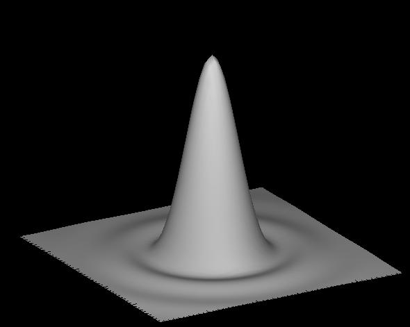
What happens if the telescope is not ideal? An image of a point source
would not be as good as Airy function, the resolution would be
degraded even more. But the imaging equation will still be
valid! So, the Point Spread Function (PSF)
![]() is
all we need to know to characterize the imaging. The width of PSF is a
measure of resolution.
is
all we need to know to characterize the imaging. The width of PSF is a
measure of resolution.
Note 1. Implicitly, we assumed in the above equations that
![]() is an image of a star of unit intensity, i.e. the
integral of
is an image of a star of unit intensity, i.e. the
integral of
![]() over
over ![]() is equal to 1. Thus, the
imaging equation preserves the total flux of an astronomical object,
only distributes it differently between the pixels.
is equal to 1. Thus, the
imaging equation preserves the total flux of an astronomical object,
only distributes it differently between the pixels.
Note 2. We assumed that PSF has the same shape over the whole field of view. This condition is called isoplanatism. It is not always true in astronomical imaging, particularly with Adaptive Optics, because PSF slowly changes in the field. In this case imaging equation can be applied to parts of the field.
The shape of PSF may be irregular; what numeric measures of resolution are used in this case?
1. FWHM = Full Width at Half Maximum of the PSF.
2. Strehl ratio
![]() , i.e. the central intensity of
PSF compared to the central intensity of the Airy function. The higher is
Strehl ratio, the better is resolution. Diffraction-limited image is the
best, hence
, i.e. the central intensity of
PSF compared to the central intensity of the Airy function. The higher is
Strehl ratio, the better is resolution. Diffraction-limited image is the
best, hence ![]() always.
always.
3. Encircled energy. By definition, the integral of PSF
is equal to 1. The PSF integral over the circle of radius
![]() is called the encircled energy. This characteristic is
important for observations of faint objects, when one wants to
concentrate the photons as much as possible.
is called the encircled energy. This characteristic is
important for observations of faint objects, when one wants to
concentrate the photons as much as possible.
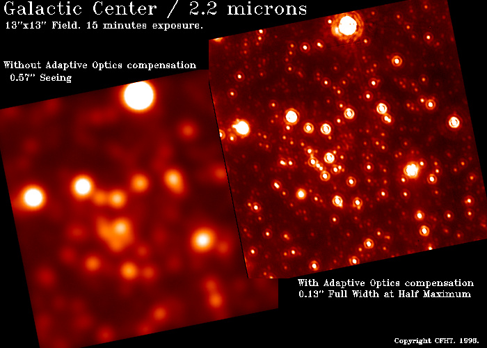
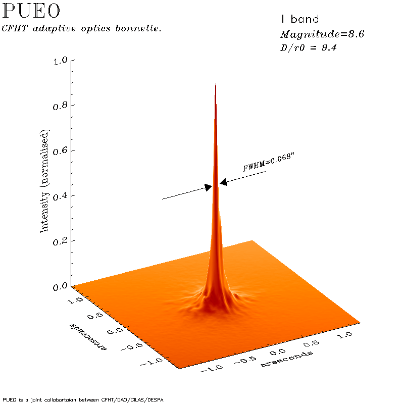
The example of the PSF with compensation of turbulence is given in the picture below.
Question: Supposing that PSF is two times narrower, by how much the Strehl ratio would change?
Question: What would be the Strehl ratio if one half of the
(ideal) telescope objective is given a phase delay of ![]() ?
?
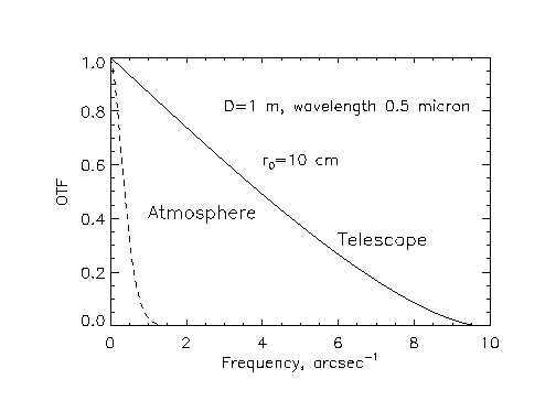
Another way to look at the imaging equation is to use the Fourier Transforms (FT; we denote it by tilde). The convolution becomes a product, so
| (3) |
The
![]() is called Optical transfer function
(OTF). It describes the change of the modulus and phase of the object
FT in the imaging process. The modulus of OTF is called
Modulation transfer function (MTF). For astronomical (incoherent)
imaging,
is called Optical transfer function
(OTF). It describes the change of the modulus and phase of the object
FT in the imaging process. The modulus of OTF is called
Modulation transfer function (MTF). For astronomical (incoherent)
imaging,
![]() . Typically, MTF decreases with
increasing frequencies, hence the small (high-frequency) details in
the image are weakened and eventually lost.
. Typically, MTF decreases with
increasing frequencies, hence the small (high-frequency) details in
the image are weakened and eventually lost.
It is known that for any optical system
![]() for
for
![]() , where
, where
![]() is called cutoff
frequency, and
is called cutoff
frequency, and ![]() is the maximal size of aperture. It means that the
information at the spatial frequencies above
is the maximal size of aperture. It means that the
information at the spatial frequencies above ![]() is irrevocably
lost. We need larger telescopes to look at smaller objects!
is irrevocably
lost. We need larger telescopes to look at smaller objects!
The relation between PSF and OTF is Fourier transform, so if you know
one you know another, they are the same thing expressed
differently. From the FT properties it follows that
![]() (PSF normalization), and that the Strehl ratio is proportional to the
integral of OTF over frequencies.
(PSF normalization), and that the Strehl ratio is proportional to the
integral of OTF over frequencies.
Question: What is the minimum size of a telescope needed to resolve a fence with 10 cm bar spacing from a distance of 5 km?
 Atmospheric turbulence may be regarded as random phase aberrations
added to the telescope. These aberrations constantly change in time, so
does the PSF. Here we consider the average PSF, corresponding to long
exposure times. The theory leads to the expression
Atmospheric turbulence may be regarded as random phase aberrations
added to the telescope. These aberrations constantly change in time, so
does the PSF. Here we consider the average PSF, corresponding to long
exposure times. The theory leads to the expression
| (4) |
The atmospheric OTF is related to the statistics of atmospheric phase
aberrations, the so-called phase structure function
![]() (see the next section):
(see the next section):
| (5) |
Question: Suppose that the shape of the atmospheric PSF is Gaussian. What is the corresponding shape of the structure function?
Question: Is the shape of the atmospheric PSF sensitive to the
structure function in the regions where
![]() and
and
![]() ?
?
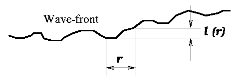
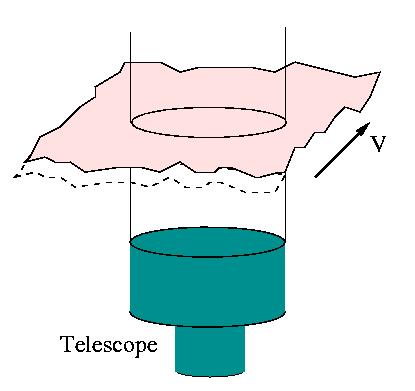
The atmospherically distorted wave-front can be visualized as a smashed paper sheet. The wave arriving from a star is plane before entering the atmosphere. Then some parts of it go through the hotter-than-average air (less refractive index) and are advanced, other parts are retarded, and the plane wave-front is deformed. It is the purpose of Adaptive Optics to compensate these distortions. But first, we need to describe them in a statistical sense.
Air is slightly dispersive, but this is usually neglected, so that the
perturbations of the optical path length ![]() are considered
as achromatic. However, the phase of the optical wave
are considered
as achromatic. However, the phase of the optical wave
![]() strongly depends on
the wavelength
strongly depends on
the wavelength ![]() ! Speaking of perturbations, we assume that
their average values are zero,
! Speaking of perturbations, we assume that
their average values are zero,
![]() (angular
brackets denote statistical averaging).
(angular
brackets denote statistical averaging).
Although random processes like ![]() are typically described
by correlation functions or covariances, in the atmospheric science
the structure functions are preferred. Structure function is
the average difference between the two values of a random process:
are typically described
by correlation functions or covariances, in the atmospheric science
the structure functions are preferred. Structure function is
the average difference between the two values of a random process:
| (6) |
Question: What is the relation between the structure function
and the covariance function
![]() ?
?
Question: How does the atmospheric
![]() depend on the
wavelength
depend on the
wavelength ![]() ?
?
 The Kolmogorov model of the turbulence distortions prescribes
the specific form of the phase structure function, namely
The Kolmogorov model of the turbulence distortions prescribes
the specific form of the phase structure function, namely
 |
(7) |
The above model, although it may seem primitive, is the basis of the whole theory of imaging through the turbulence, including Adaptive Optics. Of course, at large distances (more than few meters) and small distances (less than 1 cm) the model is not good, but this turns out to be not very important.
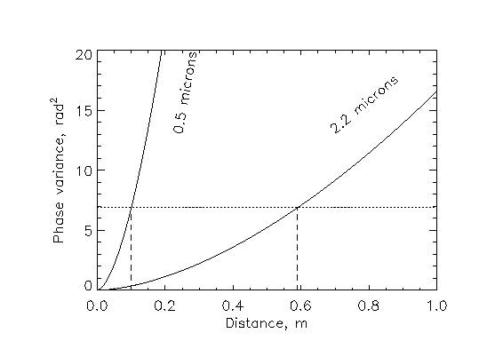
Question: What is the r.m.s. (root-mean-square) atmospheric phase
difference at the baseline of ![]() in radians and wavelengths?
in radians and wavelengths?
Question: If ![]() cm at 0.5 micron wavelength, what is
cm at 0.5 micron wavelength, what is
![]() at 2.2 micron wavelength?
at 2.2 micron wavelength?
Now we put this model into long-exposure atmospheric OTF, and get it in the form:
| (8) |
| (9) |
The Strehl number of the atmospheric PSF is exactly the same as in an
ideal telescope of diameter ![]() (this is the reason why a strange
coefficient 6.88 appears). So, for a large telescope,
(this is the reason why a strange
coefficient 6.88 appears). So, for a large telescope, ![]() ,
the Strehl ratio is simply
,
the Strehl ratio is simply ![]() .
.
Question: What is the Strehl ratio of long-exposure images at the 4 m telescope under 1 arcsecond seeing at the wavelengths of 0.5 and 2.2 microns?
The Fried radius ![]() is sometimes identified with the characteristic
scale of atmospheric perturbations. This is not quite true: we see
that Kolmogorov law does not have any characteristic scale. However,
only the perturbations of the size of the order of
is sometimes identified with the characteristic
scale of atmospheric perturbations. This is not quite true: we see
that Kolmogorov law does not have any characteristic scale. However,
only the perturbations of the size of the order of ![]() are relevant
for long-exposure imaging. At smaller scales, the distortions are much
less than
are relevant
for long-exposure imaging. At smaller scales, the distortions are much
less than ![]() , at larger scales the
, at larger scales the ![]() becomes so large
that the atmospheric OTF is zero.
becomes so large
that the atmospheric OTF is zero.
Locally, the strength of turbulent fluctuations of refractive index in
the air are described by a refractive index structure constant
![]() which is measured in strange units, m
which is measured in strange units, m![]() . The dependence
of
. The dependence
of ![]() on altitude is called the turbulence profile. Seeing
depends on the integrated effect of all atmospheric layers:
on altitude is called the turbulence profile. Seeing
depends on the integrated effect of all atmospheric layers:
| (10) |
 .
.
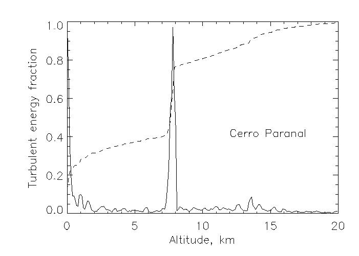
This figure shows an example of the turbulence profile at Cerro Paranal, plotted in relative units (full line). The fraction of the turbulent energy up to a given altitude is overplotted in dashed line. Although in this instance a significant part of turbulence was concentrated in only two laters, still some 1/3 of the total energy is distributed continuously over all altitudes.
Question: From this relation, find how ![]() and seeing depend
on the zenith angle
and seeing depend
on the zenith angle ![]() .
.
 Turbulence can often be modeled as fixed phase screens which are
driven by the wind in front of the telescope. Knowing the spatial
properties of the phase screens (structure function) and the wind
velocity, we know also the temporal behavior of the
perturbations. The atmospheric time constant
Turbulence can often be modeled as fixed phase screens which are
driven by the wind in front of the telescope. Knowing the spatial
properties of the phase screens (structure function) and the wind
velocity, we know also the temporal behavior of the
perturbations. The atmospheric time constant ![]() is defined
as
is defined
as
| (11) |
Question: Taking the typical value of ![]() =20 m/s, what
would be the atmospheric time constant at 0.5 and 2.2 micron
wavelengths under 1 arcsecond seeing?
=20 m/s, what
would be the atmospheric time constant at 0.5 and 2.2 micron
wavelengths under 1 arcsecond seeing?
The images of astronomical objects taken with exposure time ![]() or shorter are called short-exposure images. They correspond to
fixed (frozen) atmospheric aberrations. At longer exposure times, the
aberrations are averaged, and for exposures much longer than
or shorter are called short-exposure images. They correspond to
fixed (frozen) atmospheric aberrations. At longer exposure times, the
aberrations are averaged, and for exposures much longer than
![]() the long-exposure PSF is obtained.
the long-exposure PSF is obtained.
 The long-exposure atmospheric PSF is independent of the viewing
direction (isoplanatic), because the turbulence and its structure
function are statistically the same everywhere in the field. But the
instantaneous atmospheric phase aberrations do depend on the
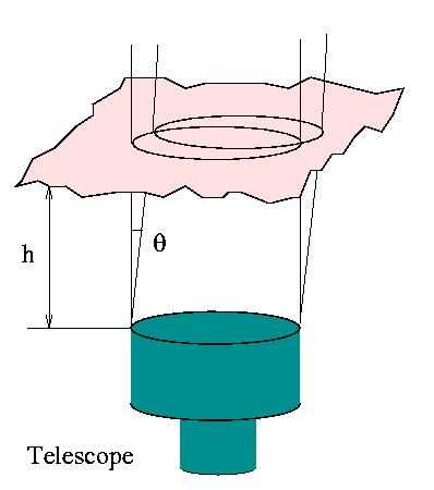
direction: the telescope beam as projected on the atmospheric layer at
10 km shifts by 0.5 m for an angular offset of 10 arcseconds.
The long-exposure atmospheric PSF is independent of the viewing
direction (isoplanatic), because the turbulence and its structure
function are statistically the same everywhere in the field. But the
instantaneous atmospheric phase aberrations do depend on the
direction: the telescope beam as projected on the atmospheric layer at
10 km shifts by 0.5 m for an angular offset of 10 arcseconds.
The standard definition of the atmospheric isoplanatic angle
![]() is
is
|
|
(12) |
Question: What is the isoplanatic angle ![]() at
wavelengths of 0.5 and 2.2 micron under 1 arcsecond seeing?
at
wavelengths of 0.5 and 2.2 micron under 1 arcsecond seeing?
This phenomenon is very troublesome for Adaptive Optics, because it limits the distance between guide star and the scientific objects. It turns out that for most objects there is no suitable (bright and close-by) guide star, hence artificial laser guide stars are required. Alternatively, a 3-dimensional correction of turbulence ( Multi-Conjugate Adaptive Optics, MCAO) may be attempted to increase the corrected field.
In optics, the aberrations are often represented as a sum of special polynomials, called Zernike polynomials. Atmospheric random aberrations can be considered in the same way; however, the coefficients of these aberrations (defocus, astigmatism, etc.) are now random functions changing in time.
A Zernike polynomial
![]() is defined in polar coordinates
is defined in polar coordinates
![]() on a circle of unit radius
on a circle of unit radius ![]() . They are characterized
by a radial order
. They are characterized
by a radial order ![]() and an azimuthal order
and an azimuthal order ![]() (for a given
(for a given
![]() ,
, ![]() takes the values from 0 to
takes the values from 0 to ![]() ). Frequently, instead of two
indices
). Frequently, instead of two
indices ![]() and
and ![]() a continuous numeration with single index
a continuous numeration with single index ![]() is
used. For a given radial order
is
used. For a given radial order ![]() , there are a total of
, there are a total of
![]() Zernike polynomials.
Zernike polynomials.
The first Zernike modes are named as common aberrations, and have simple meaning (see the Table of the first 15 Zernike modes).
The power of Zernike modes comes from the fact that they are
orthonormal, that is the scalar product ![]() is equal to 1 if
is equal to 1 if
![]() and zero otherwise. The scalar product is defined as integral
over telescope aperture:
and zero otherwise. The scalar product is defined as integral
over telescope aperture:
| (13) |
Now, any phase aberration
![]() inside the telescope pupil
can be represented as an infinite sum of Zernike polynomials
inside the telescope pupil
can be represented as an infinite sum of Zernike polynomials
 |
(14) |
| (15) |
Often a limited number of Zernike modes gives already a good enough representation of atmospheric aberrations. If these modes are corrected by Adaptive Optics, an almost diffraction-limited image quality is obtained.
Piston mode corresponds to a constant phase, which does not influence image. Usually the piston mode is ignored.
Question: A 4 m telescope, ![]() , is defocussed by 1
mm. Compute the resulting aberration
, is defocussed by 1
mm. Compute the resulting aberration ![]() for wavelengths of 0.5 and
2.2 microns.
for wavelengths of 0.5 and
2.2 microns.
Question: Suppose that atmospheric aberration contains only
random tips and tilts with equal amplitudes
![]() . Write the corresponding phase structure
function.
. Write the corresponding phase structure
function.
The orthonormality of Zernike modes gives an easy way to compute the
phase variance integrated over the pupil. For one mode, it is
![]() . The variance for all modes is equal to the sum of squared
coefficients starting from 2 (piston excluded).
. The variance for all modes is equal to the sum of squared
coefficients starting from 2 (piston excluded).
Given the Kolmogorov turbulence model, we can obtain the statistical
properties of the coefficients ![]() corresponding to the atmospheric
phase aberrations. The mathematical manipulations lead to a simple
formula:
corresponding to the atmospheric
phase aberrations. The mathematical manipulations lead to a simple
formula:
 |
(16) |
| i \ j | 2 | 3 | 4 | 5 | 6 | 7 | 8 | 9 | 10 |
| 2 | 0.449 | 0 | 0 | 0 | 0 | 0 | 0.0142 | 0 | 0 |
| 3 | 0 | 0.449 | 0 | 0 | 0 | 0.0142 | 0 | 0 | 0 |
| 4 | 0 | 0 | 0.0232 | 0 | 0 | 0 | 0 | 0 | 0 |
| 5 | 0 | 0 | 0 | 0.0232 | 0 | 0 | 0 | 0 | 0 |
| 6 | 0 | 0 | 0 | 0 | 0.0232 | 0 | 0 | 0 | 0 |
| 7 | 0 | 0.0142 | 0 | 0 | 0 | 0.00619 | 0 | 0 | 0 |
| 8 | 0.0142 | 0 | 0 | 0 | 0 | 0 | 0.00619 | 0 | 0 |
| 9 | 0 | 0 | 0 | 0 | 0 | 0 | 0 | 0.00619 | 0 |
| 10 | 0 | 0 | 0 | 0 | 0 | 0 | 0 | 0 | 0.00619 |
As you may see, the Noll matrix is almost diagonal (less so for higher
orders, however). Why the coefficient ![]() is missing? For
Kolmogorov turbulence it is infinite! However, the first (piston) mode
is of no importance to imaging.
is missing? For
Kolmogorov turbulence it is infinite! However, the first (piston) mode
is of no importance to imaging.
Question: For 4m telescope and 1 arcsecond seeing, compute the r.m.s. amplitude of tilt in radians (for 0.5 micron wavelength). Convert it to the r.m.s. amplitude of stellar image motion. Does this amplitude depend on the wavelength?
What happens if we correct the first modes with Adaptive Optics? The
corresponding coefficients become zero, and the total phase variance
is reduced. Denoting the pupil-averaged phase variance as
![]() , we write
, we write
 |
(17) |
The full, uncorrected atmospheric phase variance (all modes except
piston) corresponds to
![]() .
In other words, in a
telescope with aperture diameter of
.
In other words, in a
telescope with aperture diameter of
![]() the atmospheric phase
variance is about 1 square radians.
If tip and tilt are
corrected, then
the atmospheric phase
variance is about 1 square radians.
If tip and tilt are
corrected, then
![]() . It means that tip and tilt
contribute 87% of the total phase variance. Correcting the modes up
to radial order 2 leaves us with
. It means that tip and tilt
contribute 87% of the total phase variance. Correcting the modes up
to radial order 2 leaves us with
![]() , the radial order
3 leaves uncorrected variance of
, the radial order
3 leaves uncorrected variance of
![]() . As you see,
further reduction of phase variance demands the correction of larger
and larger number of Zernike modes.
. As you see,
further reduction of phase variance demands the correction of larger
and larger number of Zernike modes.
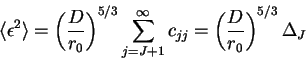
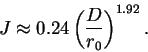
For a large number of corrected modes ![]() (
(![]() , as happens in real
systems), the assymptotic formula of Noll is very useful:
, as happens in real
systems), the assymptotic formula of Noll is very useful:
| (18) |
Question: Using the values of ![]() and
and ![]() given
above, compute
given
above, compute ![]() .
.
How many modes do we need to correct? Opticians know that when the
residual phase is less than 1 radian, the image quality approaches the
diffraction limit. You have by now all the tools to predict the
required number of modes as a function of telescope diameter, seeing,
and wavelength! It is sufficient to write
![]() and to work back all the formulas ( try to do it!). The
result is
and to work back all the formulas ( try to do it!). The
result is
 |
(19) |
Question: How many Zernike modes must be corrected at the 4 m telescope for imaging at 0.5 and 2.2 microns under 1 arcsecond seeing?
Is it necessary to correct the turbulence using Zernike modes? Of course not, the phase aberrations can be measured and corrected with any other set of basis functions, or without any modes at all, operating directly on the wave-fronts. It turns out that Zernike modes are the second best choice (the best set of modes is called Karunen-Loeve modes). The choice depends on the number of controlled parameters (modes) needed to achieve a given degree of correction; for Zernike modes it is less than for local wave-front control.
Summary. In this chapter, the fundamentals of imaging in ideal
and aberrated telescopes were reminded (PSF, OTF, diffraction limit,
Strehl ratio). Then the basic atmospheric parameters relevant for
Adaptive Optics (phase structure function, seeing, ![]() , time constant and isoplanatic angle)
were introduced. The de-composition of the random phase aberrations on
Zernike modes was studied. Now we are able to predict the number of
modes that need to be corrected.
, time constant and isoplanatic angle)
were introduced. The de-composition of the random phase aberrations on
Zernike modes was studied. Now we are able to predict the number of
modes that need to be corrected.
TOP: Introduction
FORWARD: Deformable mirrors