Top: Introduction
Forward: Wave-front sensors
Suppose that all atmospheric aberrations with scales ![]() and larger
(i.e. low-order modes) are corrected. What will be the structure
function of the remaining (residual) aberrations? Qualitatively,
it will grow at distances
and larger
(i.e. low-order modes) are corrected. What will be the structure
function of the remaining (residual) aberrations? Qualitatively,
it will grow at distances
![]() and will saturate at larger
distances at a level of
and will saturate at larger
distances at a level of
![]() (twice the
residual phase variance).
(twice the
residual phase variance).
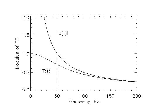
The optical transfer function, OTF, is proportional to
![]() . Instead of falling to zero at large
frequencies
. Instead of falling to zero at large
frequencies
![]() , it will become constant at the
level of
, it will become constant at the
level of
| (1) |
At large telescopes ![]() the PSF of a partially corrected
image can be represented approximately as a sum of seeing-limited
image (halo)
the PSF of a partially corrected
image can be represented approximately as a sum of seeing-limited
image (halo) ![]() and a diffraction-limited core
and a diffraction-limited core ![]() :
:
| (2) |
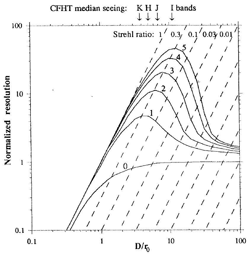
An example of a partially corrected stellar image (typical of Adaptive
Optics PSF) is given in the Figure. At large telescopes ![]() the halo is very wide compared to the core. Hence, the central
intensity of the PSF is dominated by the core and the Strehl ratio is
equal to coherent energy,
the halo is very wide compared to the core. Hence, the central
intensity of the PSF is dominated by the core and the Strehl ratio is
equal to coherent energy,
![]() . This approximation is
widely used, and sometimes
. This approximation is
widely used, and sometimes ![]() is taken as an equivalent of the
Strehl ratio.
is taken as an equivalent of the
Strehl ratio.
Question: What Strehl ratio
corresponds to the residual phase variance of 1 rad![]() ?
What is the upper limit on the residual variance needed to achieve a
Strehl ratio of 95%?
?
What is the upper limit on the residual variance needed to achieve a
Strehl ratio of 95%?
Question: Suppose that we know the Strehl ratio at a wavelength of 0.5 micron. Can you compute it at another wavelength, say 2.2 micron?
It is very important to realize that correction of large spatial
scales has an effect on small scales too, because it removes the
wave-front slopes. Hence, the structure function of the residual phase
grows less fast than the structure function of uncorrected atmospheric
aberrations. If the structure function is less, the OTF is higher, and
the PSF is narrower. The width of the halo ![]() is less than
the width of the seeing-limited PSF. This gain in FWHM can reach a
factor of 2. Even for very low Strehl ratio the improvement in the
resolution brought by Adaptive Optics can be valuable. This happens
when low-order adaptive systems are used for observations in the
visible spectral range.
is less than
the width of the seeing-limited PSF. This gain in FWHM can reach a
factor of 2. Even for very low Strehl ratio the improvement in the
resolution brought by Adaptive Optics can be valuable. This happens
when low-order adaptive systems are used for observations in the
visible spectral range.
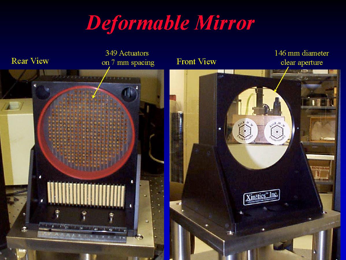
Early deformable mirrors (DMs) consisted of discreet segments, each
controlled by 3 piezoelectric actuators. Nowadays, a common technology
is to bond a thin faceplate to an array of piezoelectric actuators
(see the Figure). The actuators are not produced individually, but
rather a multi-layer wafer of piezo-ceramic is separated into
individual actuators. This type of DMs is used in the GEMINI AO
systems.
| Number of actuators | 100 - 1500 |
| Inter-actuator spacing | 2-10 mm |
| Electrode geometry | rectangular or hexagonal |
| Voltage | few hundred V |
| Stroke | few microns |
| Resonant frequency | few kHz |
| Cost | high |
Question: What is the physical size of a 1000-actuator DM with a 5 mm inter-actuator spacing?
Question: What stroke (in micrometers) is needed to correct 2 arcsecond seeing at the 4 m telescope? Suppose that tip and tilt are corrected by a separate mirror.
This type of DMs was developed primarily for military applications, they are expensive. Some examples can be found at the WEB pages of Xinetics or Turn, Ltd. Piezoelectric actuators have a hysteresis of about 10%. The maximum deformation (stroke) is limited by a saturation of the piezoelectric material (sometimes, the applied voltage is also limited). The deformable mirror of the Keck AO is shown below.
When some voltage ![]() is applied to the
is applied to the ![]() -th actuator, the shape
of DM is described by the influence function
-th actuator, the shape
of DM is described by the influence function ![]() multiplied by
multiplied by ![]() . It resembles a bell-shaped (or Gaussian) function
for DMs with continuous face-sheet (there is some cross-talk between
the actuators, typically 15%). When all actuators are driven, the
shape of the DM is hence equal to
. It resembles a bell-shaped (or Gaussian) function
for DMs with continuous face-sheet (there is some cross-talk between
the actuators, typically 15%). When all actuators are driven, the
shape of the DM is hence equal to
| (3) |
A multi-channel high-voltage amplifier is necessary to drive a piezoelectric DM. It must have a short response time, despite a high capacitive load of DM electrodes.
A bimorph mirror consists of two piezoelectric wafers which are bonded together and are oppositely polarized (parallel to their axes). An array of electrodes is deposited between the two wafers. The front and back surfaces are connected to ground. The front surface acts as a mirror.
When a voltage is applied to an electrode, one wafer contracts and the opposite wafer expands, which produces a local bending. The local curvature being proportional to voltage, these DMs are called curvature mirrors.
A tricky characteristic of bimorph DMs is that they are controlled not
in surface shape, but in surface curvature. For the same applied
voltage ![]() , the amount of the deformation produced is proportional to
, the amount of the deformation produced is proportional to
![]() , where
, where ![]() is the spatial size of the deformed
region. Similarly, the saturation of the piezoelectric ceramic must be
specified not in terms of surface stroke, but in terms of maximum
curvature (or voltage).
is the spatial size of the deformed
region. Similarly, the saturation of the piezoelectric ceramic must be
specified not in terms of surface stroke, but in terms of maximum
curvature (or voltage).
The geometry of electrodes in bimorph DMs is radial-circular, to match best the circular telescope apertures with central obscuration. In this way, for a given number of electrodes (i.e. a given number of controlled parameters) bimorph DMs reach the highest degree of turbulence compensation, better than segmented DMs.
The DM surface shape as a function of applied voltages must be found from a solution of the Poisson equation which describes deformation of a thin plate under a force applied to it. The boundary conditions must be specified as well to solve this equation. In fact, these DMs are made larger than the beam size, and an outer ring of electrodes is used to define the boundary conditions - slopes at the beam periphery.
A very simplified view of Poisson equation is the following. Curvature
is described by a Laplacian operator (the sum of second derivatives
over ![]() and
and ![]() ). In the Fourier space, Laplacian corresponds to the
multiplication by
). In the Fourier space, Laplacian corresponds to the
multiplication by ![]() . If
. If
![]() is the
Fourier transform of the voltage distribution, then the deformation
is the
Fourier transform of the voltage distribution, then the deformation
![]() is
is
| (4) |
The distribution of wavefront deformations over spatial frequencies
depends on the turbulence model. For Kolmogorov model, the amplitude
increases at low frequencies as
![]() , almost to the
-2 power of frequency. It means that the amplitude of voltage that
we need to apply to a DM will be almost independent of frequency. In
this sense, bimorph DMs are ``well matched'' to turbulence.
, almost to the
-2 power of frequency. It means that the amplitude of voltage that
we need to apply to a DM will be almost independent of frequency. In
this sense, bimorph DMs are ``well matched'' to turbulence.
Question: Suppose that turbulence is too strong and the DM approaches a saturation limit. At which spatial frequencies will the saturation occur first, at low or at high ones? Will this answer change for a segmented DM?
The mechanical mounting of a bimorph DM is delicate: on one hand, it must be left to deform, on the other hand it must be fixed in the optical system. Typically, 3 V-shaped grooves at the edges are used.
Bimorph DMs were developed on the incentive of F. Roddier for
astronomical applications, as a cheap alternative to segmented
DMs. They are used in the AO systems at CFHT, Subaru, Gemini-North
(provisionally), ESO VLT. The number of actuators remains limited.
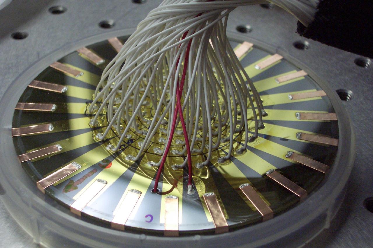
Bimorph DMs are made by CILAS in France and by Laplacian Optics in U.S.A., as well as by some other companies. Picture of a bimorph DM, view from the back side.
| Number of actuators | 13 - 85 |
| DM size | 30-200 mm |
| Electrode geometry | radial |
| Voltage | few hundred V |
| Resonant frequency | more than 500 Hz |
| Cost | moderate |
New technologies for deformable mirrors are urgently needed. To correct turbulence at extremely large telescopes (30-100 m in diameter) in the visible, DMs with 10000 - 100000 actuators will be required! One possible way to produce such DMs lies in the silicon technology (so-called MOEMS = Micro-Opto-Electro-Mechanical Systems). These DMs are made by micro-lithography, in a way similar to electronic chips, and small mirror elements are deflected by electrostatic forces. The remaining problems of MOEMS are insufficient stroke and a too small size of elements. Examples at the MEMS Optical page.
Small continuous-membrane mirrors with electrostatic control made by silicon technology are already available on the marked. They are very cheap. The number of actuators does not exceed 50, however, and a single membrane is fragile.
Another way to control the phase of light consists in using liquid crystals, like in the displays which have up to million controlled elements. Until recently, liquid crystals were too slow, but now this drawback seems to have been overcome. Still, the phase shifts introduced by liquid crystals remain too small and wavelength-dependent.
Astronomers always dreamed of correcting turbulence with deformable secondary mirrors of their telescopes, to make AO systems as simple and efficient as possible. The Figure below shows a 30-element prototype deformable secondary (SPIE, V. 4007, P. 524-531, 2000).
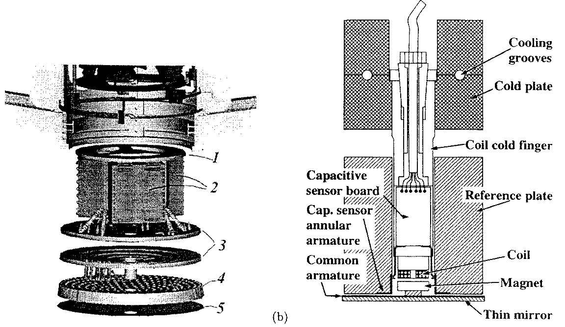 Now a deformable secondary with 336 elements is ready for the 6.5 m
MMT telescope. It consists of a thin (~1 mm) aspheric glass shell and a
thick glass base. Coils are embedded in the base, and small magnets
are glued to the shell. The gap between the shell and the base is only
few tens of microns (air in the gap damps the resonances). The shape
of the shell is controlled by an array of capacitive sensors which are
related to coils in the closed-loop system. The control of such
multi-parameter system is very complex, but finally a response time of
1.5 milliseconds was achieved. Needless to say that such DMs are
very expensive.
Now a deformable secondary with 336 elements is ready for the 6.5 m
MMT telescope. It consists of a thin (~1 mm) aspheric glass shell and a
thick glass base. Coils are embedded in the base, and small magnets
are glued to the shell. The gap between the shell and the base is only
few tens of microns (air in the gap damps the resonances). The shape
of the shell is controlled by an array of capacitive sensors which are
related to coils in the closed-loop system. The control of such
multi-parameter system is very complex, but finally a response time of
1.5 milliseconds was achieved. Needless to say that such DMs are
very expensive.
Question: Can you suggest another original ways to make DMs?
Adaptive optics works in closed loop: the WFS measures any remaining deviations of the wave-front from ideal and sends the corresponding commands to the DM. This is why small imperfections of DM (like hysteresis or static aberrations) are not very important: they will be corrected automatically, together with atmospheric aberrations. Here we consider the temporal control of the closed loop.
Let ![]() be the input signal (e.g. a coefficient of some Zernike
mode),
be the input signal (e.g. a coefficient of some Zernike
mode), ![]() - the signal applied to the DM, and
- the signal applied to the DM, and
![]() - the error signal as measured by the wave-front sensor (WFS). The
error signal must be filtered before applying it to DM, otherwise the
servo system would be unstable. In the frequency domain this filter
- the error signal as measured by the wave-front sensor (WFS). The
error signal must be filtered before applying it to DM, otherwise the
servo system would be unstable. In the frequency domain this filter
![]() is called open-loop transfer function.
is called open-loop transfer function.
To compute the reaction of the system in closed loop, we write the control equations in frequency (Fourier transform) domain:
| (5) |
 |
|||
 |
(6) |
The most common example of an open-loop transfer function is pure
integrator. The control signal is computed as an integral of error
signal with some coefficient ![]() called gain (gain must be
measured in inverse time units, like frequency). The open- and
closed-loop transfer functions for a pure integrator are
called gain (gain must be
measured in inverse time units, like frequency). The open- and
closed-loop transfer functions for a pure integrator are
 |
|||
 |
(7) |
We would like to control our DM as fast as possible to follow the changing atmospheric aberrations. In practice there are two obstacles to overcome:
1. Response time. It takes a certain time to measure the
wave-front signal by the WFS. So, ![]() gets multiplied by a delay
term
gets multiplied by a delay
term
![]() for a delay of
for a delay of ![]() . Similarly, a certain
time is spend in computing the control signal (another delay), the DM
response is not instantaneous either due to its resonances and
hysteresis (hysteresis is modeled by a constant phase lag). In short,
. Similarly, a certain
time is spend in computing the control signal (another delay), the DM
response is not instantaneous either due to its resonances and
hysteresis (hysteresis is modeled by a constant phase lag). In short,
![]() accumulates additional phase delays with increasing frequency,
and eventually the delay becomes larger than
accumulates additional phase delays with increasing frequency,
and eventually the delay becomes larger than ![]() . It means that
instead of compensating the errors, the servo system would amplify
them. If the modulus of the closed-loop transfer function at this
frequency exceeds 1, the system will become unstable. Practically, the
closed-loop bandwidth is only 1/7 to 1/10 of the lowest DM resonance
frequency.
. It means that
instead of compensating the errors, the servo system would amplify
them. If the modulus of the closed-loop transfer function at this
frequency exceeds 1, the system will become unstable. Practically, the
closed-loop bandwidth is only 1/7 to 1/10 of the lowest DM resonance
frequency.
2. Noise. The error signal is measured by the WFS with some noise. Depending on the brightness of the guide star, on the atmospheric time constant and on the correction order, an optimum bandwidth must be selected which ensures the best performance of an AO system. Practically, the loop is re-optimized during the observations. It is so complicated that we do not want to go into more details here.
We considered the signals ![]() and
and ![]() as continuous functions,
whereas in reality they are computed numerically with a certain
sampling frequency (so-called loop frequency). The theory of
digitally controlled servo systems contains some additional
complications. In practice the loop frequency must be at least 4
times higher than the closed-loop bandwidth.
as continuous functions,
whereas in reality they are computed numerically with a certain
sampling frequency (so-called loop frequency). The theory of
digitally controlled servo systems contains some additional
complications. In practice the loop frequency must be at least 4
times higher than the closed-loop bandwidth.
Question: If we need to reduce the closed-loop bandwidth twice, how shall we change the integrator gain?
Question: By how much a static aberration will be reduced by a servo system with integrator?
Question: Try to compute the closed-loop transfer function for a combination of integrator with delay and to study the loop stability conditions.
As we have seen, the ability of a DM to compensate phase aberrations is imperfect for two reasons: the limited number of actuators and the time response.
The limited capability to fit a wave-front with a finite actuator
spacing leads to the fitting error: the small details of
wave-front remain uncompensated. For an inter-actuator spacing ![]() ,
the fitting-error phase variance is
,
the fitting-error phase variance is
| (8) |
The total number of controlled actuators is ![]() , so the
fitting error is also equal to
, so the
fitting error is also equal to
| (9) |
If our DM were able to reproduce exactly ![]() Zernike modes, the
fitting error would be given by the Noll asymptotic formula. The power
index in this formula is
Zernike modes, the
fitting error would be given by the Noll asymptotic formula. The power
index in this formula is
![]() , to be compared
to
, to be compared
to
![]() in the above formula. For a large number of
controlled parameters, correcting Zernike modes gives better results
than correcting wave-fronts locally. This is why the bimorph DMs
(which can reproduce Zernike modes more closely) are more efficient
than segmented DMs.
in the above formula. For a large number of
controlled parameters, correcting Zernike modes gives better results
than correcting wave-fronts locally. This is why the bimorph DMs
(which can reproduce Zernike modes more closely) are more efficient
than segmented DMs.
It has been shown that the residual phase variance arising from the limited bandwidth of a servo system is approximated as
| (10) |
In fact the temporal spectrum of Zernike coefficients depends on the order of mode: low-order modes change less rapidly. It makes sense to control each mode with a different response time, optimized for a minimal residual error in the presence of WFS noise. This approach is called modal control and is implemented in some AO systems.
Question: Suppose that the
maximum degradation of the Strehl ratio due to control bandwidth is
specified to be 0.9. Which ![]() is needed to achieve
this goal if
is needed to achieve
this goal if ![]() is 4 ms?
is 4 ms?
Question: For the case of
Gemini (![]() m) and 1 arcsecond seeing, compute the
required number of segmented-mirror actuators to achieve a Strehl
ratio of 0.37 at 0.5 micron wavelength, and the number of corrected
Zernike modes needed to achieve the same Strehl ratio.
m) and 1 arcsecond seeing, compute the
required number of segmented-mirror actuators to achieve a Strehl
ratio of 0.37 at 0.5 micron wavelength, and the number of corrected
Zernike modes needed to achieve the same Strehl ratio.
Summary. Now we know how to compute the quality of partially compensated image (Strehl ratio) and how to select the number of controlled parameters. The present and future choices of deformable mirrors were reviewed, and the fundamentals of closed-loop control were introduced. We have formulas to compute the residual phase errors arising from finite actuator spacing and from finite response time of the servo.
TOP: Introduction
FORWARD: Wave-front sensors