| basic numbers | picture here |
A reference manual describing the spectrograph optics, gratings, camera, CCD, etc.
The R-C grating spectrograph is used at the f/7.8 R-C focus of the V.M. Blanco 4.0-m telescope where the scale is 6.56 "/mm. It is identical in design to the one at Kitt Peak National Observatory and, as far as possible, in operation. The distinguishing feature of these spectrographs is their large beam size (point-source beam size is 152mm). As a result, higher dispersion than usual for Cassegrain spectrographs is available, along with excellent spatial resolution for observations of extended objects. All functions of the spectrograph can be controlled remotely by the data acquisition computer, permitting convenient and efficient operation.
This is a basic walk-through of the spectrograph. Refer to the optical diagram below. The basic elements (in the order they get hit by incoming photons) are:
|
Slit/Decker Filter Collimator Grating Camera & CCD |
 [1] [1] |
kfnxc,kfjvfnd;ghregjth
Acquisition & Guiding [2]
Description of the Field Acquistion and Slit Viewing TV & the Offset Guider
R-C Spectrograph Slit & Decker
The entrance slit has a length of 50 mm. Its width has a range from closure to 50 mm. One second of arc corresponds to approximately 150µ and, with the Blue Air Schmidt camera and Loral 3K×1K CCD now used with the R-C spectrograph, a 1" slit projects to 2 pixels on the CCD for small grating tilts. Because of anamorphic magnification, the 2-pixel projected slit width will be greater than 150µ at large grating tilts. Here is a plot showing the 2-pixel projected slit width as function of grating angle readout.
The decker plate for defining the length of the slit is normally left in the fully open position. With the decker fully open, the field of view is limited to 50 mm, 328 arcseconds, by the length of the slit. For reference the other available decker positions are:
| No. | mm | arcsec | |
| 1 | 1.86 | 12 | |
| 2 | 3.71 | 24 | |
| 3 | 7.42 | 49 | |
| 4 | 14.85 | 97 | |
| 5 | 30.98 | 203 |
Michael Keane (mkeaneATnoao.edu)
Jack Baldwin (jbaldwinATnoao.edu)
Two filter bolts that each can hold four filters and a clear position are available. The lower filter bolt contains neutral density filters; the upper filter bolt contains either order-sorting [3] filters or additional neutral density filters. An additional filter holder for a single order-sorting [3] filter can be manually inserted into the beam if required.
Note that any filters used are all located behind the slit, and so will alter the collimator focus. The final collimator focus value should be determined with the desired filters in place.
Michael Keane (mkeaneATnoao.edu)
Jack Baldwin (jbaldwinATnoao.edu)
The collimator mirror is an off-axis (11°) paraboloid of 225mm diameter and 1161mm focal length. The point-source beam size is 152mm.
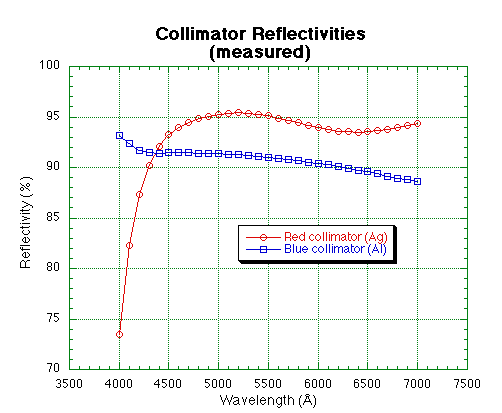
There are two collmators available for the R-C spectrograph on the Blanco 4-m, the "blue" collimator and the "red" collimator. The difference is that the blue collimator is Aluminium coated, while the red is silver coated.
NOTE: As of 20 Apr 2000, the red collimator is not available because the coating was damaged. We are investigating recoating it, but in the mean time, only the blue collimator is available.
The plot below shows the last measured reflectivities of the two collimators.
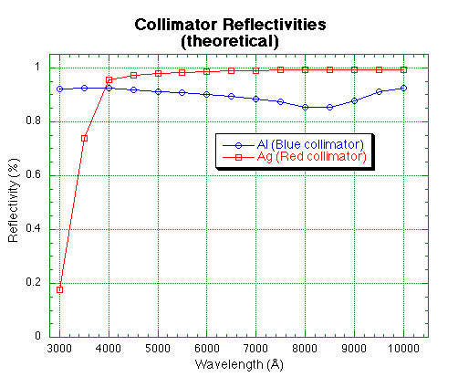
Just for reference, the following plot and table show the catalog reflectivities for Ag and Al over the optical spectral range. This shows the theoretical best performance of the two coatings, NOT the real values.
Last update: April 24, 2000
Chris Smith (csmithATnoao.edu)
Knut Olsen (kolsenATnoao.edu)
The 4.0-m R-C spectrograph has a fixed 46° angle between the optical axes of the collimator & camera. For sufficiently large grating tilts e.g., observing at high dispersion, the beam coming from the collimator can overfill the grating resulting in the loss of a small amount of light. For the 4.0-m R-C spectrograph, the collimated beam begins to overfill the grating for tilts > ~30.3° (readout < ~36.6°).
The amount of light which may be lost due to overfilling the grating is almost always neglible, typically a few percent. In practice, this small loss would be more than offset by the abliity to observe using a wider slit while preserving spectral resolution that results from the anamorphic demagnification [4] at large grating tilts.
At present, there are thirteen 203×254 mm gratings available. Their nominal specifications are listed below, along with dispersion, and coverage in 1st order available with the BAS + L3K.
| 1st Order | |||||
|---|---|---|---|---|---|
| Grating | l/mm |
Blaze [1] (A) |
Wavelength Coverage (A) |
Dispersion
(A/pixel) |
Notes |
| G250 | 158 | 4000 | 11431 | 3.75 | |
| G400 | 158 | 8000 | 11431 | 3.75 | 2 |
| G510 | 300 | 10000 | 5999 | 2.01 | 2,3 |
| G181 | 316 | 7500 | 5708 | 1.91 | |
| KPGL2 | 316 | 4400 | 5708 | 1.91 | |
| KPGL3 | 527 | 5500 | 3417 | 1.16 | |
| G420 | 600 | 8000 | 2981 | 1.02 | 3 |
| KPGL1 | 632 | 4200 | 2872 | 0.95 | |
| KPGLF | 632 | 8200 | 2872 | 0.95 | |
| G450 | 632 | 11000 | 2872 | 0.95 | |
| KPGLD | 790 | 8500 | 2290 | 0.75 | |
| KPGLG | 860 | 11000 | 2101 | 0.68 | |
| G380 | 1200 | 8000 | 1563 | 0.48 | 3 |
Notes:
                                                       R-C Spectrograph
                                                Grating Relative Efficiencies

Grating:  250  400   510  181 KPGL2 KPGL3 420 KPGL1 KPGLF  450  KPGLG   KPGLD    380
Lines/mm: 158  158   300  316   316   527 600   632   632  632    860     790   1200
   Blaze:4000 8000 10000 7500 4400 5500  8000  4200  8200 11000  11000    8500   8000
Wavelength:                           Blue-blazed gratings relative to grating 250 [5]
   3250  1.00                 1.13                  0.77     			       3250
   3500  1.00 0.04            1.14   0.38   0.76II  0.78                               3500
   3750  1.00 0.10 0.64II     1.14   0.52   0.71II  0.83                               3750
   4000  1.00 0.26 0.79II     1.17   0.70   0.73II  0.97                               4000
   4250  1.00 0.45 0.83II     1.20   0.86   0.64II  1.04        0.73II                 4250
   4500  1.00 0.66 0.81II     1.17   1.08   0.58II  1.11        0.71II                 4500
   4750  1.00 0.89 0.76II     1.25   1.29   0.43II  1.21        0.81II		       4750
   5000  1.00 1.16 0.72II     1.24   1.42   0.34II  1.29        0.98II         0.67II  5000
   5250  1.00 1.40 0.62II     1.28   1.58   0.27II  1.34			       5250
   5500  1.00 1.64 0.66II     1.31   1.66           1.40			       5500
   5750  1.00 1.92 0.57II     1.25   1.71           1.36			       5750
   6000  1.00 2.14 0.58II     1.29   1.88           1.44			       6000
   6250  1.00 2.47 0.49II     1.18   2.02           1.47			       6250
   6500  1.00 2.65 0.36II     1.14   2.11					       6500
   6750  1.00 2.85 0.38II     1.12   2.15					       6750
   7000  1.00 3.18 0.35II     1.20   2.31                                              7000

Grating: 250  400   510   181 KPGL2  KPGL3 420 KPGL1 KPGLF  450  KPGLG   KPGLD   380

 II signifies second order.


Grating:  250  400   510  181 KPGL2 KPGL3  420 KPGL1 KPGLF  450  KPGLG  KPGLD   380
Lines/mm: 158  158   300  316   316   527  600   632   632  632    860    790  1200
   Blaze:4000 8000 10000 7500  4400  5500 8000  4200  8200 11000  11000  8500  8000
Wavelength:                           Red-blazed gratings relative to grating 400 [6]
   5000  0.86 1.00 0.62II      1.06  1.22 0.37II 1.11				       5000
   5250  0.71 1.00 0.45II      0.91  1.13 0.24II 0.96				       5250
   5500  0.61 1.00 0.40II      0.80  1.02 0.17II 0.86				       5500
   5750  0.52 1.00 0.30II      0.65  0.89        0.71            0.69II		       5750
   6000  0.47 1.00 0.27II      0.60  0.88        0.67            0.62II		       6000
   6250  0.41 1.00 0.20II      0.48  0.82 1.05   0.60      1.05  0.54II 0.74	       6250
   6500  0.38 1.00 0.14II 1.03 0.43  0.80 1.04             1.01  0.45II 0.75  0.46     6500
   6750  0.35 1.00 0.14II 0.96 0.40  0.76 0.99             0.97  0.39II 0.77  0.50     6750
   7000  0.32 1.00 0.11II 0.90 0.38  0.73 0.89             0.93  0.38II 0.77  0.48     7000
   7250  0.30 1.00 0.91   0.91 0.35  0.70 1.01             0.90         0.89           7250
   7500  0.27 1.00 1.00   0.90 0.32  0.67 1.04             0.86         0.90           7500
   7750  0.27 1.00 1.00   0.86 0.32  0.69 1.01             0.84         0.95           7750
   8000  0.26 1.00 1.05   0.89       0.67 1.00             0.82         1.02           8000
   8250  0.24 1.00 1.14   0.90       0.64 1.02             0.81  0.46   1.09           8250
   8500  0.26 1.00 1.13   0.90            1.03             0.81  0.54                  8500
   8750  0.23 1.00 1.14                                    0.84  0.60                  8750
   9000  0.25 1.00 0.99                                    0.92                        9000
   9250  0.27 1.00 0.98                                    1.08			       9250
   9500       1.00 1.09                                    1.11			       9500
   9750       1.00 1.20                                    1.16			       9750
  10000       1.00										     	     10000

Grating: 250  400  510  181  KPGL2 KPGL3  420 KPGL1  KPGLF  450  KPGLG  KPGLD   380

 II signifies second order.
Michael Keane (mkeaneATnoao.edu)
Jack Baldwin (jbaldwinATnoao.edu)
Only one camera and CCD combination is presently used with the R-C spectrograph: the Blue Air Schmidt (BAS) and Loral 3K CCD (L3K). The Air Schmidt camera is a field-flattened Schmidt camera of 229 mm focal length and 229 mm clear aperture (f/1). This camera is used exclusively with the Loral 3K CCD, which together with its special dewar, forms an integral part of the camera.
The Local 3K [7] is a thinned 3K×1K CCD with 15µ pixels. The CCD has a two layer AR coating and is UV flooded to maximise its QE [8] over a wide range of wavelengths.
The demagnification with the BAS is a factor of 5.1 which results in a spatial scale of 0.50 arcsecond per 15micron pixel. The full field of view illuminated by the 50mm long slit [9] is approximately 656 pixels or 328 arcseconds.
Michael Keane (mkeaneATnoao.edu)
Jack Baldwin (jbaldwinATnoao.edu)
Updated April 1 1997.
The new Loral 3K CCD plus Blue Air Schmidt combination was first tested with the 4.0-m RC spectrograph during an engineering run on 15-16 February 1995. This is a thinned 3K x 1K CCD with 15 micron pixels. The CCD has a two layer AR coating and is UV flooded to maximise its QE over a wide range of wavelengths. It is flat.
All indications are that it is superior in all respects to both the Blue Air Schmidt + Reticon and the Folded Schmidt plus Tek1024. In particular we believe it to be the best choice of CCD for all the CS CCD runs in the present block of observing time.
The Loral 3K has two working amplifiers (lower left LL and lower right LR). However only one can be used at a time. We have set up the two video channels to have almost a factor two difference in gain, to allow the user more freedom of choice. Looking at the table below, it can be seen that LL is better optimized given that the full-well capacity is only 78000 e-. (ie LL, gain 2, gives 1.99 e/adu, 7.7 e- RON, and full well will occur at 39000 ADU). UNFORTUNATELY, the high video gain needed for LL has meant that LL suffers from some stability problems (noise bands, bias drifts) and FOR THE MOMENT, we recommend using the LR amp, at gain 4. The only advantage of gains 1,2,3 with LR is readout speed, use these gain settings only if readout time is critical for your program.
i ARCON 3.5 / Loral 3K
n Full CCD
d DCS __Read_Noise___ ____1/Gain___ __Read_Noise__ SingleRead
e (us) (ADU) (e-/ADU) (e-) Time (s)
x LL LR LL LR LL LR
------------------------ -------------- --------------- ----------
1 5 2.54 1.48 4.33 7.82 11.0 11.6 88.2
2 10 3.88 2.17 1.99 3.96 7.7 8.6 120.5
3 15 5.68 2.97 1.39 2.59 7.5 7.7 152.4
4 20 7.08 3.87 1.03 1.94 7.3 7.5 184.4
Dark current is extremely low, 0.48 e-/pixel/hour
QE and System Efficiency:
The QE of the CCD (measured at KPNO) is:
Wavelength QE (%)
3200A 78.9
3650A 73.9
4050A 73.0
5000A 86.6
6000A 93.0
7000A 93.9
8000A 73.9
9000A 41.8
There has been some scepticism expressed that the QE figures below 3000A are very optimistic. We do not yet have any really definitive measurements of our own, but figures of around 30-40 % at 3500A may be nearer the truth. The below system efficiency figures assume that the KPNO QE measurements are correct.
The overall system efficiency (fraction of photons striking the primary mirror which are detected by the CCD) was measured using standard stars. Using grating KPGL1 (632 l/mm 4200A blaze) and a wide (10") spectrograph slit the measured efficiency was:
Wavelength Loral3K Reticon
3000A 2.4%
3500A 10.6% 8.0%
4000A 14.1% 9.6%
5000A 18.6% 10.4%
6000A 14.3% 8.1%
The third column gives values for the Reticon #2 CCD using the same grating.
Image quality:
With a very narrow (50 mu slit which projects to 0.6666 pix), and at best focus, the measured FWHM of comparison lines is 2.3 pix. For a slit width of 150 mu (2 pix, 1.0") the best FWHM grows to ~2.6 pix, while at 225 mu (3 pix, 1.5") it is ~3.0 pix. There is slight curvature of the focal plane which results in some variation of the FWHM with position on the CCD. With the 150 mu slit the images are 3.3 pix FWHM or better over most of the chip (~4 pix in the extreme corners), while with a 225 mu slit the images are 4.5 pix or better over most of the chip (~5 pix worst case). Even the worst case images are quite symmetrical, and do not show the very broad assymmetric wings seen in out of focus images obtained with the Reticon (B A/Sch) and Tek1k (F/Sch CCDs. In general the images obtained with the Loral are much more uniform than with these other CCDs.
Gratings:
The gollowing table lists the coverage and dispersion (A/pix) obtained with the various gratings available for the R-C spectrograph. It is also valid for the Argus multiple object spectrograph.
| Grating | l/mm |
Blaze % (A) |
Cover. (A) |
Dispn. (A/pix) |
Notes |
| 250 | 158 | 4000 | 11431 | 3.75 | |
| 400 | 158 | 8000 | 11431 | 3.75 | * |
| 510 | 300 | 10000 | 5999 | 2.01 | *# |
| 181 | 316 | 7500 | 5708 | 1.91 | |
| kpgl2 | 316 | 4400 | 5708 | 1.91 | |
| kpgl3 | 527 | 5500 | 3417 | 1.16 | |
| 420 | 600 | 8000 | 2981 | 1.02 | # |
| kpgl1 | 632 | 4200 | 2872 | 0.95 | |
| kpglf | 632 | 8200 | 2872 | 0.95 | |
| 450 | 632 | 11000 | 2872 | 0.95 | |
| kpgld | 790 | 8500 | 2290 | 0.75 | |
| kpglg | 860 | 11000 | 2101 | 0.68 | |
| 380 | 1200 | 8000 | 1563 | 0.48 | # |
% Littrow value: for the actual RC spectrograph configuration the effective
blaze wavelength is 0.92 of the Littrow value.
* This grating is silver coated and so does not reflect light below ~ 4000A
# This grating is not very efficient when used in second order.
This CCD fringes redward of about 7000A. The maximum fringe amplitude is +/-1% which occurs at a wavelength of ~8500A. The fringe spaceing is ~40 pixels. Note that the fringe amplitude for the Loral is less than that for the Reticon (+/- 3-4%). We do not yet know how well the fringes are corrected by flat fielding. The spectrograph flexes by less than 2.5 pixels or 0.06 of a fringe spacing from the zenith to +/- 5h HA. Thus dome flat fields obtained with the white spot will probably be adequate for fringe correction in many cases. Note that dome flats can be obtained at two telescope/dome positions: North 0H, +20d 40m, dome pa 218; and South 0H, -81d 00m, dome PA 039. It may help to use the flat field position according to the declination of your objects.
Nonethless, until more experience has been obtained, we recommend that users working redward of 7000A and requiring better than 1% flat fielding obtain quartz flats (using the same slit width as for the object) for each object.
Note that it is possible to switch between Ne and Quartz lamps under software control. Set the manual switch on the comparison lamp in the cage to the "Quartz position" and select Ne as the comparison lamp in setspec/instrpars. The Ne lamp will automaticaly be selected for exposures of type comp and the quartz lamp for pflats.
Steve Heathcote (sheathcoteATnoao.edu)
Alistair Walker (awalkerATnoao.edu)
This manual covers the ARCON-IRAF software interface that is used for acquiring images and controlling the spectrograph.
A Preliminary User's Guide
13 April 1994
This is a preliminary guide to using CTIO's new CCD controller, Arcon, in conjunction with the 4.0-m RC Spectrograph to obtain spectroscopic data.
Both the hardware and software for Arcon are still under development and are consequently a little buggy. This manual is pretty buggy too. The mountain Observer Support staff, have, as yet, little experience with the system and thus will be less able to help with problems than is usual, and will often have to refer to the "experts" in La Serena. Please bear with us during this transition phase. But please also be diligent about reporting any problems and bugs you may encounter and please feel free to make any suggestions or criticisms you may have.
The IRAF based user interface allows observing commands to be sent to Arcon from within the IRAF cl. This results in a single uniform user interface for data taking and data reduction and allows the Arcon user to employ features of the cl such as the parameter mechanism and the history editor. It also allows advanced users to write cl scripts which freely mix data acquisition and data reduction operations. It is nonetheless simple enough, that users need very little knowledge of IRAF in order to obtain their data. As far as possible the user interface is modeled on the ICE software in use at KPNO; the present manual also owes more than a little to the KPNO ICE manual. However, users should be aware that the two systems are NOT identical, so that parameter lists may differ and data acquisition scripts written for ICE will require some modification.
Figure 1 shows a block diagram of the various computers and peripherals which make up the data acquisition system at a typical CTIO telescope. You should find a version of this diagram for your specific telescope, showing the names of the actual computers and peripherals involved, posted in the console room. At least some of the key pieces of hardware are labeled; if you have trouble locating, for instance, the exabyte drive, at your telescope ask observer support.
In the console room of the 4.0-m telescope you will find two Sun Computers. One of these, a SPARC-station 10/41, is the Arcon data acquisition computer. You must log on to this machine in order to use Arcon and, in general, will also want to use it for all your data reduction. The other machine is an older VME-bus based Sun 4/330; currently peripherals such as the 9-track and exabyte tape drives and laser printer are attached to this second Sun. If more than one observer is present at the telescope, or if you find a single Sun screen to be too restrictive, you may wish to use this second machine for your reductions. However, if you do so we recommend you treat it as an "intelligent terminal" from which you log on to the data acquisition machine. Accessing images across the network imposes a very stiff penalty in the form of increased I/O overheads when reducing your data.
When you first log on to the data acquisition computer using your visitor account, you will be asked which windowing system you prefer -- both Sunview and Openwindows are available -- as follows(1):
- What windowing system do you want?
0 -- No windowing system
1 -- SunView
2 -- OpenWindows
Enter selection (1): 1
Pick whichever you are most comfortable with, or select SunView if you know neither (in this case you may want to refer to Appendix C). The system remembers your answer, so you will only be asked to make this choice the first time you log on to a given machine. You will then be asked if you want to start up the data acquisition program, or just to reduce data as follows:
- What type of IRAF setup do you want?
1 -- IRAF for data reduction
2 -- IRAF with Arcon
Enter selection (1): 2
If you select "2", as in the example, your chosen window system will start up and several windows will open so that your screen should look something like Figure 1; the function of these various windows will be explained in Section 2.2. An automatic start-up procedure will also be run which initialize the controller hardware and software. This takes some time; when it finishes the message "Array Controller ready for user commands ..." will appear along with a beep. Wait until you see this message and hear the beep before continuing.
At present there are a few additional steps which you must carry out manually by typing the following in the specified windows (as a reminder, the necessary commands are shown in the parentheses in the title bars of most of these windows):
In the window labeled Arcon STATUS: type astro1_up
In the very small green window: type countdown
The IRAF cl will automatically start up in the blue window labeled "IRAF, Acquisition (arcon......)". You must first load the arcon package, and then the specific package for the instrument you are using -- csccd for Cassegrain focus CCD spectroscopy. To do so proceed as follows:
ar> csccd
Connecting to the controller...
abort dflat maskfocus preview shutter
comp disconnect more recover specseq
compin enablespec movie restorespec stop
compout gainchange object resume tchange
connect initspec observe savespec teloffset
dark instrpars@ obspars@ setspec telpars@
detector instrument pause sflat ufbolt@
detpars@ lfbolt@ pflat showspec zero
Loading the instrument package automatically establishes the connection to the controller, as indicated by the "Connecting to the controller...." message hidden amongst the package menus. Exiting from the package with bye or (usually inadvertently!) ctrl-z breaks the connection.
You are now ready to start taking data. However, before you begin doing so in earnest, you should check that everything is set up and working properly: (i) Check you know where your home directory is (show home); (ii) Check where your imdir is (show imdir), that it really exists (cd imdir) and that you have the necessary privileges (copy home$login.cl imdir$junk; delete imdir$junk); (iii) check there is plenty of disk space (disks); (iv) carry out the basic tests of the operation of the detector and controller described in the instrument manual. If there are problems with any of this seek help from observer support.
A further word about image directories is in order at this point. Each of the data acquisition machines has several 2-3Gb capacity disks for bulk data storage. On each of these there will be a directory, /iraf, containing sub-directories for each visitor account. At the start of your run all these disks will be cleared. However, especially if you are using the Tek2048 CCD, you will have no trouble filling the available space in a few nights of typical observing. From time to time you should use the command disks to see how much space is free on each disk. Arcon uses the value of the IRAF environment variable imdir in order to decide where to write the pixel files for newly created images.
You can change the value of this variable "on the fly" with the command
cl> reset imdir = /ua12/iraf/v19/
Note that the trailing "/" character is necessary. This variable will be restored to its original default value when you log out of IRAF. Also the values in the acquisition and reduction windows are independent and must be set separately. To change imdir permanently and insure the two windows use the same value, you must edit your .cshrc file as follows,
cl> edit home$.cshrc
# DEFAULT OBSERVER/VISITOR CSHRC FILE.
..........
# Image pixel directory definition. This is the ONLY place where this
# variable should be defined and changed.
setenv imdir "/ua12/iraf/$USER/" <----- Change this line as required
You must then log out of IRAF and back in again, for the change to take effect.
Once you have completed the initialization procedure, your screen should appear similar to Figure 2. The key windows for taking data with Arcon, identified by the names given in their title bars, are as follows:
Arcon CONSOLE -- As its name implies this window serves as a console for Arcon. While you are observing you will see many messages appear here, only some of which will be repeated in the IRAF acquisition window. This window takes up a lot of screen space so you will probably prefer to close it. But don't quit from it. In the event that something goes wrong, the diagnostic messages appearing in this window may tell you (or at least us) what happened.
Arcon STATUS -- This very important window gives several lines of information summarizing the status of the controller, the instrument, and any ongoing exposures (see Figure 3). The first line shows what the controller is currently doing. if you have just brought the system up, it should read "CONTINUOUSLY_ERASING" indicating that the CCD is idle and is continuously running the erase cycle; if it doesn't, chances are something went wrong in the initialization and you should seek help. During exposures this line should read "INTEGRATING", and should change to "READING" as the CCD is read out. Other messages which may occur will be described later as appropriate. Just below the status line are counters showing the number of seconds left in the current exposure, the number of exposures left in the current sequence, and, during read out, the number of buffers of data successfully transferred to the Sun. Also shown are parameters of the current exposure such as the title, picture name etc. Finally the bottom three lines of the status window show, during readout, the values of various statistics of the image. These numbers are generated on the fly by the real time display program (see Section 6) and are used in setting the display look up table. You, however, may find this information useful when adjusting exposure times during sequences of sky flats, etc.
COUNTDOWN --This is the very small window with the very large font. It provides a copy of the exposure time counter for the visually handicapped.
IRAF Acquisition -- This blue colored window is one of two running the IRAF cl. We recommend you type all data taking commands here, so that your data taking and data reduction activities are well separated and don't interfere with one another.
IRAF Reductions -- This window (colored a dirty brick red) is the other IRAF window. We suggest that normal IRAF commands, used to examine or reduce your data are entered in this window.
IRAF Display Window -- depending on your choice of window environment there will be either an
"SAO Image" (Open Windows) or "Imtool" (Sun View) window which will be used when displaying your images from IRAF.
Before you log out, for whatever reason, you must first stop the various processes, related to the controller running on the Sun. If you don't do this they will continue running and cause all sorts of entertainment for you or whoever else next tries to bring up the system. To do so first, in the blue "IRAF, Acquisition" window, break the connection to the controller by either typing disconnect or by exiting from the instrument package by typing bye. Then in the "Arcon CONSOLE" window type:
arsh> arsh stop
ctioa1% kleenex
This last command should clean-up all the processes related to Arcon; unfortunately it doesn't always. To see if it worked type:
% NexUp
No match.
No match.
No match.
If you get "No match." three times in a row, as above, all is well. If instead you see something like
ctioa1% NexUp
root 2227 0.0 3.0 2664 844 p6 S 17:32 0:05 muxnex
arcon 2229 0.0 .6 172 160 p2 S 17:32 0:00 arsh -c 0 -e 20
arcon 2228 0.0 .0 144 0 p2 IW 17:32 0:00 arsh -c 0-e20
/dev/nexc0
Nomatch.
-rw--rw- 1 arcon 0 Jul 13 17:32 /tmp/xpim2229.1
-rw-rw-rw- 1 arcon 0 Jul 13 17:33 /tmp/xpim2245.1
then there are some leftover processes which you must kill by hand as follows,
ctioa1% kill -9 2227 2229 2228
In this command the list of numbers after the -9 are the pid's of the leftover processes as displayed by NexUp. The files with names like /tmp/xpim2229.1 are the spool files used by Arcon to transfer data to the Sun. If any of these are owned by you and have a size other than zero (the number just before the date), then they may contain your missing data! See section 3.1.2 for information on how to retrieve this. It is common to see a few zero length files as shown in the example, but these can be ignored.
Now you can exit from the windowing system and log out completely, by moving the mouse to a blank area of the screen, then hold down the right mouse button, and select "exit" from the menu which will appear.
Rather more often than we would like, currently about once a night, something or other happens which causes the system to hang requiring that the software be reloaded.
Before doing so it is worth testing to see if the problem is confined to the IRAF interface layer, by proceeding as follows:
co> flpr
co> disconnect
Disconnecting from Nexus ....
co> connect
Connecting to Nexus ....
co> flpr
This re-establishes and initializes the connection to the Arcon and, for good measure, flushes out any brain-damaged executables locked into the IRAF process cache. Having done this, test to see if the problem has gone away by taking a "zero" frame.
If this fails, or if the status window or real time display have stopped functioning, then the problem is probably in Arcon itself and it is best to reload the software from scratch. This takes very little time. First follow the steps in Section 2.3 for shutting down the system, but do not perform the very last step of exiting from the window system. Instead restart the Arcon software as follows:
In Arcon CONSOLE type arcon_visitor, then wait until you see the message "Array Controller ready for user commands ..." and hear a beep before continuing.
In Arcon STATUS type astro1_up or simply "!!"
In green font window type countdown or simply "!!"
In the blue IRAF window type connect or reload the instrument package (cfccd, pfccd, nfccd)
Also in the IRAF window type setdetector force+ to ensure that all parameters of the detector match the values you have selected in the detpars pset (see Section 5.3)
Just once in a while a problem will occur which just refuses to go away even when you reload the Arcon software. This may be due to a hardware failure. However, it may also be that the Sun has got irremediably confused, in which case the rather drastic step of rebooting it may be called for. Should this prove necessary contact observer support. They can show you how to reboot the Sun safely, cleanly, and without having to know the superuser password.
All data taking can be done by using a single command: observe. This command takes one or more ccd exposures, as in the following example:
cs> observe
Exposure type (|zero|dark|object|dflat|sflat|pflat|comp|) (comp): obj
Number of exposures to take (1:) (3): 1
Exposure time (0.:) (5.): 600
Have you switched OFF the lamp ?????!!!!!
compout
comparison lens OUT enabled
Title of picture (comp at ngc1097): ngc1097 nuc
cs>
Image obj060 written to disk
Observation finished...
You will be prompted for all the information required which includes:
exposure type: can be "zero" (sometimes referred to as bias), "dark", "object", "dflat", "sflat" or "comp" (used for taking comparison lamp exposures). Note that when selecting from a list of options like this you may enter any unique abbreviation as shown in the example.
number of exposures to take: a sequence of this number of pictures, all having the same parameters, will be taken.
exposure time: is in seconds, and will not be requested in the case of exposures of type "zero" for which it is 0.0 by definition.
picture title will be included as the title in the IRAF image header.
Note that in each parameter query you will be supplied with a default value, which you can accept by simply hitting <cr>; these values are just the previous entries.
If you make a mistake, or change your mind, you can abort the command during the parameter entry stage by typing ctrl-c; having done so you should always enter the command flpr, as a means of warding off the evil eye. Once the exposure has started it can be terminated using the abort command (see Section 3.2).
The program automaticaly sets the comparison optics appropriately for the type of exposure being taken: for exposures of type "comp" and "pflat" the mirror carriage in the instrument rotator will be moved to the comparison position ("mirror 4") and the comparison lens will be moved into the beam; for exposures of types "object", "dflat" and "sflat" the rotator mirror is moved to the object position ("mirror 2") and the comparison lens is moved out of the beam; for exposures of type "zero" and "dark" these mechanisms are not moved. Currently the comparison lamps must be turned on and off manually with a switch located near the observer's position. The program prints out a reminder to do this. These hardware actions are performed between the prompts for the exposure time and the title.
As soon as you enter the title, the CCD will be prepared, and then the exposure will begin. The first line in the status window will change from "CONTINUOUSLY_ERASING" to "INTEGRATING" and the status window will also show parameters of the exposure such as the picture title. A counter in the status window, and more legibly the countdown window will begin counting down the time remaining in the exposure. At present these counters are not exactly synchronized with the internal clock in the controller so for very long exposures they may indicate that a few seconds remain when the exposure is in fact complete. A further counter in the status window will count up the dark time -- the time since the CCD stopped being erased. This may be slightly greater than the elapsed exposure time due to overheads in the controller, and will of course be very much longer if you paused the exposure.
Note that the observe command terminates as soon as the exposure starts and you can enter other commands in the IRAF acquisition window. While you could type any IRAF command you like, we suggest you keep this window free for entering the special exposure control commands described in Section 3.2
When the exposure finishes the CCD will be read out. The first line in the status window will change to "READING" and the "buffers read" counter will indicate the number of buffers of data successfully transferred to the Sun. The data is initially written in the controllers internal format to a spool file on /tmp, but it is automatically converted into an IRAF image within a few seconds of the exposure finishing. The message "Image ...... written to disk" appears as soon as this process is complete and shows you the name of the new IRAF image. This name is derived from the exposure type by appending a running number (see section 5.1 for how to adjust this number) which is automatically incremented after each exposure. The image header will be in the current directory (at the time the observe command was issued) and the pixel file will be located in your imdir.
During readout the image will also be displayed on the real time display (see Section 6). This occurs independently from and in parallel with the transfer of the data to disk on the Sun. You need not wait for the real time display to finish before starting another exposure.
If you requested that observe take only a single exposure, the message "observation finished ....." will appear in the IRAF interface window as soon as the readout is complete; things are then ready for you to start another exposure. If, instead, you requested a sequence of several pictures, the next exposure will start automatically. You may immediately examine or process the resulting image even though the sequence is not complete. Note that the "pictures remaining" counter in the status window shows how many exposures remain in the sequence. Once the final picture has been readout the message "sequence finished ......" will appear in the IRAF interface window. Should you miss the end of sequence or end of exposure message, note that the CCD is idle and things are ready for you to initiate new exposures, whenever the top line of the status display reads "continuously_erasing".
Sometimes Arcon will successfully transfer your data to the spool file on /tmp but the picread program which converts this to an IRAF image will fail. Usually there is an error message, but you should be suspicious that this has happened if the exposure completes normally, but you can't find the output image. The command recover will assist you to retrieve your valuable images in such cases. It searches /tmp for any spool files owned by you and for any of these that are complete will show the FITS header and ask if you want to recover the image or not. If you reply yes then picread will be run to convert the xpim file to an IRAF image. A single spool file occasionally contains more than one image. In this case recover will list how many images are present, but will only show you the header of the first. All images will be recovered if you tell the program to go ahead. Spool files are not removed from /tmp until successfully converted by picread. However, we suggest you run recover immediately if you encounter this problem, so that you don't forget later, and so that /tmp doesn't get filled to overflowing with unprocessed spool files.
Sometimes a failure occurs during the transfer of the data from the controller to the Sun. In this case a partial spool file results which cannot be used to resurrect the data. Recover will give you the option of deleting any such files, and you should do so to avoid filling /tmp with debris.
But, don't give up hope yet! There is a 2.5M-byte internal buffer in the controller itself, so you can still rescue your data, provided the entire image fits in this space; a Tek1024 CCD image fits, a full unbinned Tek2048 image does not. To attempt this, reload the Arcon software by following the "warm start instructions" (See Section 2.5). Wait for the message
Array Controller ready for user commands ....
then type the following in the Arcon console window:
arsh> macro NoData
Now take a picture as you normally would. The picture will be read from
the memory buffer, NOT from the CCD. Once you have done this successfully
type:
arsh> macro DetectorData
(again in the Arcon console window) to restore things to normal.
The following commands can be used to modify an ongoing exposure:
pause - Pause the exposure e.g. while waiting out passing clouds.
resume - Resume a paused exposure.
tchange - Change exposure time. You will be prompted for the amount by which to change the exposure which may be positive or negative. If used during a sequence the duration of the present exposure and all subsequent exposures is changed.
stop - Stop the exposure early, read out the CCD and save the data to disk. If used during a sequence, the sequence is also terminated.
abort - Abort the exposure. The CCD is not read out and any data collected during the exposure is irrevocably lost. If used during a sequence, the sequence is also terminated.
Note that, currently, it is not possible to cleanly terminate the process of reading out the CCD. If you issue an abort command during readout it will not take effect until the current exposure has been completely read out (i.e stop and abort are equivalent under these circumstances). For very large chips like the Tek2048, it may be faster to just re-initialize the controller (see Section 2.4).
In addition to observe, there are specific commands to take one or more pictures of each type:
comp - Take one or more comparison lamp exposures
dark - Take one or more exposures of type dark
dflat - Take one or more exposures of type dome flat
object - Take one or more exposures of type object
sflat - Take one or more exposures of type sky flat
zero - Take one or more exposures of type bias
Except, of course, for the exposure type these commands take the same parameters (and prompt for them in the same order) as does observe. Apart from saving you entering that one extra parameter, use of these commands allows one to set default parameter values, and also select which parameters are prompted for according to picture type.
Another useful command is:
more - Take one or more exposures exactly like the previous one
The more command is slightly unusual in the way it prompts for parameters (it is patterned after commands like directory and help). If you type
cf> more
you will not be prompted for the number of exposures (as one might expect) but rather a single exposure will be taken (which more often than not is what you actually wanted to do). Conversely
cf> more 10
will take ten more exposures.
Frequently one wants to take one or more exposures of the same object bracketed by comparison exposures, for instance to monitor flexure of the spectrograph. This can be done very conveniently with the command specseq as shown in the following example
cs> specseq
number of object exposures per sequence (1:) (1): 3
Number of times to repeat basic sequence (1:) (2): 1
Exposure time for object exposures (0.:) (600.):600
Title for pictures (test): NGC 1068
Have you switched ON the lamp ?????!!!!!
compin
comparison lens IN enabled
Image comp060 written to disk
Observation finished...
Have you switched OFF the lamp ?????!!!!!
compin
comparison lens OUT enabled
Image obj061 written to disk
Observation finished...
.......
This will take a comparison exposure followed by three (answer to first prompt) exposures of the object and finish up with another comparison exposure. The answer to the second prompt determines how many times this basic comparison-object-comparison sequence is to be repeated. Note that because the comparison lamp must be turned on and off manually you cannot go to sleep completely while the command is executed. This task has two hidden parameters which should be set using epar before it is run for the first time.
cs> epar specseq
I R A F
Image Reduction and Analysis Facility
PACKAGE = csccd
TASK = specseq
npics = 1 number of object exposures per sequence
nsequenc = 2 Number of times to repeat basic sequence
exposure = 600. Exposure time for object exposures
title = test Title for pictures
(comptim = 10.) Exposure time for comparison exposures
(sequenc = both) Take comparison exposures at
(mode = ql)
Comptime sets the exposure time for the comparison exposures. Sequence determines where comparison exposures should be taken in the sequence and can be set to "start", "end" or "both".
Two commands which may be useful when centering your object on the detector or for establishing rough focus, are:
preview - Take a CCD exposure and display it on the real time display but does not write any data to disk.
movie - Loop continuously taking and displaying preview exposures until terminated by stop.
Both commands prompt for a single parameter the exposure time; since the readout time in quad mode is 15-20 seconds for the Tek1024 CCD some degree of real-time feedback can be obtained using movie with exposure times of a few seconds. In the near future preview and movie will optionally use special waveforms which reduce the readout time at the expense of increased noise &/or reduced spatial resolution.
The most important functions of the 4.0-m RC Spectrograph --including the slit width, grating tilt, and collimator focus -- are motorized and can be adjusted under computer control. There are a few important and perhaps surprising exceptions; the comparison lamps have to be turned on and off using a switch near the observers positions, and one must go to the cassegrain cage in order to select between the various lamps available. Also the spectrograph camera focus is set manually in the cage.
As you might guess from the whirring and grinding noises which go on when any of these motors are moving, the hardware is antique, but it still (mostly) works. Currently the spectrograph is controlled using a program written in FORTH running on an LSI-11 (this same software is used with CTIO's VEB's). However, this has been tied in to the Arcon-IRAF interface by having the Sun send commands to the LSI-11 over a serial line. Thus data taking and spectrograph control appear to be fully integrated from the point of view of the user, and full information on the spectrograph configuration gets included in the image headers.
As described in Section 3.1 the comparison optics (rotator mirror and comparison lens) are automaticaly positioned as required whenever you take an exposure. The commands compin and compout can be used to insert or remove the comparison optics, respectively, without having to take an exposure.
The remaining components of the spectrograph are controlled by the setspec command. Executing this command will bring up a parameter editor screen as shown below
cs> setspec
I R A F
Image Reduction and Analysis Facility
PACKAGE = csccd
TASK = setspec
slitwidt = 300 Slit width (microns)
decker = open decker position
(grating = kpgl2) Grating identification
tilt = 6200 grating tilt (hundredths of degrees)
(collima = blue) Collimator identification
colfocus = 440 Collimator focus position
(camera = FoldedSchmidt) Spectrograph camera identification
camfocus = 1.2,2.4,0.,1.2 Spectrograph camera focus
ufilter = open upper filter position
lfilter = GG495 lower filter position
mask = south Newall mask / slow shutter
skysuppr = open Sky suppressor position
rsviewer = out rear slit viewer
(complamp = "HeNeAr") Comparison lamp
(mode = m)
($nargs = 0)
There is a parameter for each mechanism in the spectrograph. To reposition the corresponding motor, move the cursor up and down with the arrow keys until you are on the correct line and then simply type the new value followed by <cr>. When you are done editing the parameters type cntrl-z. All the motors you have edited will then be moved to the requested positions. For many of these motors several tens of seconds are required to move from one end of the range of travel to the other, and only one motor can be moved at a time, so be patient. If you mess up and want to exit from the command without moving any motors type cntrl-c
The parameters grating, collimator, camera, camfocus and complamp(2), do not correspond to actual motors. Changing their values will not cause anything to be moved. However, these values are recorded in the image header so you may wish to set them correctly in order to keep track of the spectrograph configuration used for each observation.
If you only want to position one or two motors a useful shortcut is to run the command as in the following example
cs> setspec slit=150 mode=h
150 slit
slit 150 enabled
where only the slit width was adjusted. The mode=h tells IRAF to run the command without bringing up the parameter editor.
To check that all the motors are positioned as you want, for instance before starting an observation, use the showspec command:
cs> showspec
Comparison lamp : off
Grating identification : kpgl2
Collimator identification : blue
Spectrograph camera identification : FoldedSchmidt
Spectrograph camera focus : 1.22,0.0,2.45,1.22
R-C Spectrograph Hardware status
sky suppressor ??? enabled
filter bolts #1 `1' enabled
#2 `1' enabled
newall mask OPEN enabled
slit viewer OUT enabled
decker OPEN enabled
slit 300 enabled
collimator 440 enabled
comparison lens OUT enabled
grating 6202 enabled
Note that there is a significant pause after the "R-C Spectrograph Hardware status" line while the program goes out and reads all the encoders. Its a good idea to run showspec from time to time to ensure that setspec has not got confused about the true configuration of the spectrograph (see Section 4.6).
If your program calls for more than one set up of the spectrograph -- for instance if you change
gratings or grating tilts during the night -- then you can save time and avoid mistakes by saving the parameters for each configuration in a file. When you have the spectrograph set up to your satisfaction type
cs> savespec red_setup
this will save the configuration in a file called red_setup (you can include a full pathname if you want this file to be somewhere other than the current directory). Subsequently you can restore the spectrograph to exactly the same configuration by typing
cs> restorespec red_setup
An important shortcoming of the present arrangement for spectrograph control is that the setspec program is not able to read the encoders in order to determine the actual configuration of the spectrograph. Rather it just remembers the last position to which it moved each motor and assumes they have not subsequently been moved by some other agency. The program will thus be fooled if the configuration of the spectrograph is changed manually, or if the motors are moved by someone logged in under a different user name. Also of course setspec has no way of knowing the initial state of the spectrograph the very first time it is run. The command initspec moves all the motors in the spectrograph so that their positions match those shown in the parameter file of the setspec command. If setspec is only confused about the position of a few motors you can initialize these individually as in the following example.
cs> initspec tilt,slit
where the grating tilt and slitwidth are the parameters to be reset.
Note that the positions of the various motors given by the showspec command are the true values as determined by reading the encoders. A mismatch between the values listed by that command and those in the setspec parameter file indicates that you need to run initspec.
As with ICE many of the nitty-gritty details of taking your data are hidden from your immediate view in four parameter files:
obspars This contains several parameters which you, the astronomer, can use to tailor the behavior of observe to your liking.
instrpars This parameter file contains information relating to the instrument being used -- the RC Spectrograph in this case.
detpars This parameter file controls the fundamentals of how the CCD is readout -- binning, gain, regions of interest, etc.
telpars The 4.0-m telescope is run by a control program which is interrogated by Arcon, at the start of each exposure, in order to obtain information such as the time, telescope coordinates, etc. for inclusion in the image header. This parameter file currently does nothing and has only been retained to maintain compatibility with ICE.
You should review these parameter files, and may want to change some values, at the start of your run, but will probably leave them alone thereafter.
These parameter files can be listed by using the lpar command, eg.,
cf> lpar obspars
and may be edited using the parameter editor, epar, or by simply typing the name of the parameter set e.g.,
cf> epar obspars -OR-
cf> obspars
To change a value, in either case, move the cursor up and down with the arrow keys until you are on the correct line and then simply type the new value followed by <cr>. When done editing the parameter file type cntrl-z
The parameter file obspars is shown below:
I R A F
Image Reduction and Analysis Facility
PACKAGE =
cfccd
TASK =
obspars
ccdtype = zero Exposure type
npics = 1 Number of exposures to take
picture = 1 Picture number of first exposure
exposure = 0. Exposure time
title = Title of picture
(autopic = yes) Generate picture number automatically ?
# POSITION COMPARISON OPTICS FOR EACH EXPOSURE
(setcomp = auto) Query and set complens & rotator mirror
(mode = ql)
($nargs = 0)
It is not necessary to set the values of the majority of these parameters, since they are prompted for as needed. The values appearing in obspars are simply the values entered the last time observe was run. The parameter autopicnum determines whether observe will prompt you for the running picture number, picture, which forms part of the name of your images on disk. The value of picture is always incremented after each exposure. If autopicnum=yes (the default) the automatically derived value will always be used and you will not be prompted. If autopicnum=no you will be prompted for a new value of picture for every exposure, the automatically derived value being supplied as the default. In either case you can reset the sequence by just changing the value of picture in obspars. Note that picture will get out of step if you abort an exposure or sequence; the value used will be the one which would have been appropriate if the exposure or sequence had completed normally.
The only other parameter you might want to change is setcomp which controls the positioning of the comparison optics at the start of each exposure. The default value "auto" will cause the comparison optics to be positioned appropriately for the type of exposure being taken as described in Section 3.1. If this parameter is set to "yes" you will be prompted for the desired position of the rotator mirror and comparison lens for every exposure. If it is set to "no" the comparison optics will not be moved at the start of the exposures although they can still be moved with the compin and compout commands.
The instrpars parameter set contains all the parameters of the spectrograph as shown below:
I R A F
Image Reduction and Analysis Facility
rotatorm= Rotator mirror position
complens= out Comparison lens
(complam= HeNeAr) Comparison lamp
(slitwid= 300) Slit width (microns)
(decker = open) decker position
(grating= kpgl2) Grating identification
(tilt = 6200) Grating tilt (hundredths of degrees)
(collima= blue) Collimator identification
(colfocu= 440) Collimator focus position
(camera = FoldedSchmidt) Spectrograph camera identification
(camfocu= 1.3,1.6,1.0,1.3) Spectrograph camera focus
(ufilter= 1) Upper filter position
(lfilter= 1) Lower filter position
(ufbolt = ) Filter info. pset for Upper filter bolt
(lfbolt = ) Filter info. pset for Lower filter bolt
(mask = south) Newall mask / slow shutter
(skysupp= open) Sky suppressor position
(rsviewe= out) Rear slit viewer
(instrna= rcspec) Instrument name
(mode = ql)
These parameters are normally changed using the commands setspec, compin and compout. You should merely verify that the last parameter instrname is set to "rcspec" and leave everything else alone.
The detpars pset holds parameters related to the CCD detector itself such as the section of the chip to be readout, the binning factors and so on. The detpars file is slightly different for each detector, because each has its own personality. At the start of your run, and before you begin customising any parameters in detpars you should do the following
cf> unlearn detpars odetpars
(N.B. there is no coma). This ensures that the private copy of the pset stored in your uparm directory is appropriate for the detector you are using. You must repeat this command if you change detectors part way through your run.
As with any pset you can edit the contents of detpars by typing epar detpars or just detpars. However, any changes you make this way will not be immediately downloaded to the controller. To make your changes effective you must run the command setdetector
cf> setdetector
this will first bring up the parameter editor allowing you to review and make any additional changes to detpars. Once you are happy exit with cntrl-z and your changes will be sent down to the controller. If you change your mind or make a mistake, and want to exit without changing anything, type ctrl-c. For some parameters only a single command is sent to the controller to change the value stored internaly. Others require that the waveforms which control the clocking of the CCD are recompiled and downloaded into the controller, a process which takes some time and generates several dozen lines of output. Eventualy when all is done the package prompt (e.g. cf>) will be output.
Normaly setdetector only downloads new parameter values to the controller if these have changed since the last time it was run. When the controller software is reloaded (by running arcon_visitor see Sections 2.2 and 2.5) the internal variables in the controller are reset to their initial values. The information stored by setdetector about the parameter values in the controller is then incorrect. A similar confusion will arise if setdetector has been run from a different account (e.g. by observer support). To force setdetector to update all parameters ensuring that everything is in sync. type
cf> setdetector force+
IMPORTANT: If you are not using the default values for all the parameters in detpars then you must do this each time you reload the controller software.
The complete detpars pset for the Tek1024 CCD is shown below:
I R A F
Image Reduction and Analysis Facility
PACKAGE = csccd
TASK = detpars
(preflas= 0.) Preflash time (seconds)
(xsum = 1) pixels summed in X direction
(ysum = 1) pixels summed in Y direction
(xstart = 1) Start of ROI in X
(ystart = 1) Start of ROI in Y
(xsize = 1024) Size of ROI in X
(ysize = 1024) Size of ROI in Y
(extend = separate) Method of extending ROI to include overscan
(noversc= 18) Number of overscan pixels (physical)
(xskip1 = 3) X pixels to skip at start of overscan
(xskip2 = 0) X pixels to skip at end of overscan
(xtrim1 = 0) X pixels to trim at start of data
(xtrim2 = 0) X pixels to trim at end of data
(ytrim1 = 0) Y pixels to trim at start of data
(ytrim2 = 0) Y pixels to trim at end of data
(amplifi= quad) Readout amplifiers to be used
(pixsize= 24.) Pixel size in microns
(nxpixel= 1024) Detector size in X
(nypixel= 1024) Detector size in Y
(detname= Tek1024-2) Detector identification
the function of the various groups of parameters are described in the following sub-sections.
Many of CTIO's CCD's have more than one, typically four, working amplifiers. A major advance achieved with Arcon is the ability to read out the CCD using more than one of these amplifiers in parallel, leading to substantially faster read-out. Once properly reduced, such data is virtualy indistinguishable from that obtained when reading out through only a single amplifier. However, raw multi-readout images do look decidedly strange(3). Firstly, each read-out will typically have a slightly different, zero level, gain, and readout noise, and may differ slightly in its departures from perfect linearity. As a result both zero frames and uniformly illuminated exposures will show a characteristic chequer board pattern, the sections of the data read through each amplifier having different levels. Secondly, there will be a separate overscan strip, used to monitor the zero level, for each readout. The location of these overscan strips within the image depends on which amplifiers are selected as illustrated in Figure ?.
The combination of amplifiers to be used is set by the parameter amplifiers. The available choices are
quad - Use all four amplifiers. The resulting image is split horizontaly and verticaly into four equal quadrants the overscan regions forming a vertical stripe down the centre of the picture.
upper, lower - Use the upper or lower pair of amplifiers. The resulting image is split in two horizontaly, the overscan strips running side by side down the centre of the picture.
right, left - Use the right hand or left hand pair of amplifiers. The resulting image is split in two verticaly. The overscan strips lie one above the other along the side of the picture furthest from the amplifiers in use ( i.e. at the left if amplifiers = right and conversely).
ll, lr, ul, ur - Use single amplifier in the lower left, lower right, upper left and upper right corner respectively. The overscan strip runs verticaly down the edge of the picture farthest from the amplifier (i.e. down the right edge for ll and ul and the left edge for lr and ur).
Theoreticaly there are another two cases, using the pairs of amplifiers at opposite corners of the chip, but we haven't had reason to impliment these yet. Not all choices are available with every CCD; enter ? as the value of amplifiers when editing detpars to see a list of the ones appropriate for the particular chip you are using.
The Thomson (Arcon 2.1 and Arcon 3.1) and Tek1024-2 (Arcon 3.2) chips each have four working amplifiers and you should in general choose quad for these detectors. Due to a broken bond wire, only the upper two amplifiers on the Tek 2048 (Arcon 3.3) can be used and one should in general select upper in this case. If the very small residual differences between the properties of the data in the segments that remain after data reduction would be a problem for your program you might wish to select a single amplifier. Consult Alistair Walker for advice on this and on which amplifier to use if you do.
This parameters sets the number of seconds for which the preflash leds should be illuminated at the start of each exposure. Currently none of the CCDs used with Arcon require a preflash, although the preflash leds are sometimes used when performing diagnostic tests on the CCD. You should in general just check that the preflash is set to 0.0 and leave it that way.
These parameters specify the number of adjacent detector pixels to be combined in the X and Y directions respectively. Use of binning is inapropriate for most spectroscopic applications.
These parameters specify the rectangular sub-section of the CCD which is to be readout (see Figure ?). The length of the spectrograph slit does not fill the full size of the detector in the spatial direction. Thus you can speed up the readout and save space on disk by only reading out the data for the part of the chip covered by the slit. If you do this you should leave a generous margin at either end of the slit to allow for measurement of the scattered light (See the CTIO cookbook CSCCD, available on line and in the red binders, for advice). The amount of time and space that can be saved in this way is small, and this is just one more thing you have to get set up properly. Therefore, our advice is that you do not do this unless the redout time overhead is a critical factor for your program (e.g. you are doing time resolved spectroscopy).
The coordinates of the bottom left hand corner of the region you want to read out are given by xstart and ystart, while its size is given by xsize and ysize. These values must be specified in physical pixels on the CCD, not binned pixels. The parameter extend controls how the region is to be extended to include the overscan strip. The default value separate causes any pixels between the trailing edge of the ROI and the overscan strip to be skipped -- this is usualy what you want. If you select extend the interveening pixels will be read out and included in the output image. If you select none there will be no overscan strip at all; this can be useful for test exposures but don't do this if you hope ever to reduced your data.
The actual portion of the CCD that will be read out will include the entire region you specify, however additional pixels may be included for a number of reasons. Firstly, if you are binning, the coordinates of the ROI will be automaticaly adjusted to be a whole number of binned pixels. Secondly, if the overscan is included by extending extra pixels will be read between the end of the region and the start of the overscan. Thirdly for some CCDs it is necessary to read a few extra gaurd pixels around the edges of the region to avoid contamination of the data by electronic transients. Finaly, if you are using more than one readout amplifier, additional pixels and/or "phantom regions" will be readout for reasons of symmetry (see Figure ?). The trimsection information recorded in the image header will be set so that all these extra pixels are excised when the image is reduced.
The parameter noverscan sets the number of overscan pixels to be read for use in determining the DC-bias level of the CCD. This parameter should be given in binned pixels. There is an overscan strip for each amplifier used so that if the CCD is split in the horizontal direction there will be twice this number of overscan pixels in total. The parameters xskip1 and xskip2 are supposed to be used in setting the biassection information in the image header (see Figure ??); xskip1 pixels will be ignored at the leading edge of the overscan strip and xskip2 pixels at the trailing edge. Unfortunately the controller is currently not doing this calculation correctly and the header values are incorrect. You must in any case overide the header values when you actualy reduce the data with quadproc. Thus you need not set these parameters now.
These parameters control the trimsection information written in the image header (see Figure ??) which is used when processing the data. These values must be given in physical CCD pixels, not binned pixels. The default values will normaly be what you want. In any case you will have the opportunity to overide the header values when you actualy reduce the data.
The final group of parameters in detpars are purely for information and you will be unable to change their values. These are intended to be read by programs which need to know information about the characteristics of the detector, but currently this information is not being used anywhere.
In Arcon the parameter which determines the number of e-/ADU is the slope time of the "double-correlated-sampler" -- usually erroneously referred to (by astronomers) as the gain. Currently, however, this is not done via entries in detpars, but rather by running the program gainchange (at least at CTIO, programmers do what astronomers tell them to do, even when its wrong), as follows:
cf> gainchange
Gain setting (0 for list) (0): 2
*** Regenerating waveforms ***
csh /pxp/run/macro/wdl Tek1K_1 -I..
WDL revision 2.18
..........
*** Suspending the sequencer ***
*** Reloading new waveforms ***
You will be prompted for the gain setting, which must currently be one of a pre-defined list of values. The CCD readout waveforms are then edited, recompiled, and down loaded into the controller. This all takes about 12s. To get the list of acceptable gain settings, and also (one day soon) to find out the corresponding number of e-/ADU, readout noise, and readout time, enter a gain setting of 0, as follows:
cs> gain 0
dcsT Delay ____Read_Noise_____ _______1/Gain______ ____Read_Noise_____ Read
T (ADU) (e-/ADU) (e-) Time
(us) LL LR UL UR LL LR UL UR LL LR UL UR (s)
--- ---- ------------------- ------------------- -----------------------
1: 9 5 1.54 1.53 1.59 1.56 3.39 4.36 4.36 4.40 14
2: 12 5 2.85 3.27 3.27 3.30 15.5
3: 15 4 2.00 1.86 1.77 1.91 2.28 2.62 2.62 2.64 4.56 4.87 4.64 5.04 17
4: 20 4 2.64 2.37 2.32 2.45 1.71 1.96 1.96 1.98 4.51 4.65 4.56 4.84 20.5: 39 4 5.49 4.26 4.45 4.37 0.88 1.01 1.01 1.02 4.82 4.29 4.48 4.43 29
^
* *** Select gain setting from the first column ***
*** Current gain setting is 4
For advice on what gain is right for you, refer to the appropriate users manual, or consult observer support.
This parameter set is not used at this time.
Arcon includes a real-time display which automatically shows each picture as it is being read out on a separate Sun-style monitor next to the data Acquisition computer. This occurs independently from, and in parallel with, the transfer of the data to disk on the Sun and does not slow down this process. You need not wait for the real time display to finish before starting another exposure. The real time display offers a number of convenient features:
Display of the picture begins substantially before all the data has been transferred to the Sun and converted into an IRAF image.
Various picture statistics are accumulated on the fly and are used to optimally map the 16-bit CCD data into the 256 grey-levels shown by the display. These statistics are also shown in the status window (see Section 2.3) and may be useful when estimating exposure levels for sky flats.
Saturated pixels (data value 65535) are shown in red.
Quad readout pictures are automatically overscan subtracted and trimmed for the display.
The cardinal directions are labeled on the display monitor. You will soon be able to specify any rotation and flipping necessary to have the display match your finding charts.
These features mean that you can always see the last picture taken to verify that the picture looks reasonable, is the field you want, and that no important objects are saturated.
The display itself takes place in two stages. A first fast pass keeps up with the readout but the data is shown at slightly reduced spatial resolution. A second, slower full resolution pass is then performed once the entire picture is available. Since the ideal mapping from 16 to 8 bits can't be known until the readout is finished the second pass may modify the look up table unless you specify otherwise (see Section 6.2).
You can change the way the mapping from 16 to 8 bits is performed and also whether the picture is shown in normal, reversed or false color mode. You can also show the pixels above and below the mapped range in green and blue, respectively. The commands to control these settings are temporarily contained in the contributed package (a sub-package of arcon):
lut - Change the look up table.
Parameters:
video = "reverse" (normal|reverse|falsecolor)
Show stars as white ("normal"), black ("reverse") or use false-color ("falsecolor").
colors = "nocolor" (nocolor|3color)
Disable ("nocolor") or enable ("3color") the use of colors to mark pixels outside the mapping range. When enabled pixels below the range are shown in blue and those above the range are shown in green. Note this does not affect the marking of saturated pixels which are always shown in red.
map - Defines the way the 16-bit CCD data is to be mapped to the 8-bit display. The default parameter values (algorithm = "mode", low = 0.2, high = 2.0) work well for normal star fields. Try low = 0.2 and high = 1.3 to bring out nebulosity.
Parameters:
algorithm = "mode" (mode|stdev|minmax|constant|show)
The mapping algorithm to use. Options are:
mode - Map range is specified number of standard deviations below mode and above mean.
stdev - Like mode, except bottom of range is specified number of standard deviations below mean.
minmax - Map range has specified percentages of pixels above picture minimum below picture maximum. (e.g. 0.5 and 1 would have 0.5% of the pixels below the map range and 1% above the map range.)
constant - Set map range to specified values.
show - Display current picture with specified values, but do not change the map parameters for subsequent picture displays.
low = 0.2
Low value for mapping algorithm. This is expressed as a number of standard deviations for the mode and stdev algorithms, the percentage of pixels below the bound for minmax and the absolute level in ADU's for constant and show.
high = 2
High value for mapping algorithm. This is expressed as a number of standard deviations for the mode and stdev algorithms, the percentage of pixels above the bound for minmax and the absolute level in ADU's for constant and show.
The 16-to-8-bit mapping is performed based on image statistics accumulated as the picture is read out. However, it is necessary to wait until enough of the picture data is available, so that these statistics are meaningful, before using them for the mapping. Until then the mapping from the previous exposure is used. This works well when sequential exposures are of the same type and comparable duration. In the future the system will be made smarter so that the preliminary mapping used is based on information from the previous exposure of the same type scaled according to exposure time.
The remap task (also temporarily in the contributed package) controls how soon remapping is performed:
remap - Set remapping options for real time display.
Parameters:
delaydisplay = no
Do not start displaying until percent of the picture has been read. This prevents starting to display pictures with the mapping from the previous picture, but delays any feedback on the current picture.
percent = 43
The percentage of the picture which must be read out before the mapping for the first display pass is changed from that used for the previous picture.
redraw = yes
Perform final high resolution display pass.
With the default value of percent repainting of the screen with the new look-up table will finish bef ore CCD read-out completes. A smaller value will result in earlier re-mapping, but an increased risk that incomplete sampling of the field will result in a poor choice of look-up table. In some cases such as when an isolated bright star or a compact star cluster are placed near the center of a quad readout detector, the correct mapping cannot be known until the end of the readout. When the new look-up table is poorly chosen, the display may be repainted three times; once at the start using the look-up table from the previous exposure, then again based on statistics accumulated from the top and bottom edges of the image, and finally when the readout is complete based on statistics from the entire picture. This final remapping is done at the same time that the image is displayed at full spatial resolution. Some people find this repeated repainting of the screen confusing. If you decide you do not want any remapping, set percent = 100. and delaydisplay = yes. Display of the picture will then not start until the read-out is complete, at which time you will see a fast, medium spatial-resolution display, followed by a second slower pass at full resolution, but there will be no change in the mapping.
Appendix A: Software Summary - The Only Page(s) You Really Need to read.
arcon - Load main Arcon package
cfccd - Load instrument specific package for Cassegrain focus CCD direct
pfccd - Load instrument specific package for Prime focus CCD direct
nfccd - Load instrument specific package for Newtonian focus CCD direct
connect - Make connection to detector controller (automatically done by cfccd etc)
disconnect - Break connection to detector controller (automatically done on bye from cfccd)
observe - Take one or more exposures prompting for type
dark - Take one or more dark exposures
dflat - Take one or more dome flat exposures
object - Take one or more object exposures
sflat - Take one or more sky flat exposures
zero - Take one or more zero exposures
focus - Take a focus frame
more - Take more exposures of the previous type
preview - Take an exposure preview frame. Data is shown on real time display but not saved to disk.
movie - Continuously take preview exposures until stopped with abort
abort - Stop exposure and do not readout detector
stop - Stop exposure and readout detector
tchange - Change exposure time
pause - Pause current exposure
resume - resume paused exposure
obspars - Observing parameters
detpars - Detector parameters
telpars - Telescope parameters
instrpars - Instrument parameters
ufbolt - filter info parameters for upper filter bolt
lfbolt - filter info parameters for lower filter bolt
initspec - Initialise spectrograph motor control and settings
setspec - Set all spectrograph settings
showspec - Show all spectrograph settings
compin - Set comparison lens & rotator mirror ready for comp or pflat
compout - Set comparison lens & rotator mirror ready for object
savespec - Save current spectrograph settings in a file
restorespec - Restore spectrograph settings from a file
Notas
1. In examples like this, text entered by the user will be shown in bold type in order to distinguish it from prompts and other output from the program.
2.In particular note that changing complamp does not select which comparison source is used. This has to be done manually in the Cassegrain cage.
3. Note that these oddities are not apparent when the data is viewed on the real time display, because this automatically trims the overscan and applies an offset and gain correction to each quadrant to crudely equalize the DC levels.
| Plate Scale (at f/7.8 focal plane) | 6.56 arcsec/mm | |
| Slit Length |
50 mm 328 arcsec |
|
| Collimator Focal Length | 1161 mm | |
| Point source collimated beam diameter | 152 mm | |
| Collimator-to-Camera Angle | 46° | |
| Grating size | 203×254 mm | |
| Camera Focal Length | 229 mm | |
| Demagnification | 5.070 | |
| Plate Scale (at detector) | 33.3 arcsec/mm |
Michael Keane (mkeaneATnoao.edu)
Jack Baldwin (jbaldwinATnoao.edu)
Several old but useful HeAr and HeNeAr comparison line atlases.
These are scanned versions of older HeAr and HeNeAr comparison line atlases which have been used at CTIO for many years. The line ratios from our lamps have changed somewhat over the years, but these are still some of the best references available for identifying HeAr and HeNeAr lamp spectra from CTIO, at least until we get around to reproducing them from more recent spectra!
HeAr, low resolution, 3800-7200A: GIF [10] - PDF [11]
HeAr, med resolution, 3000-4100A: GIF [12] - PDF [13]
HeAr, med resolution, 3800-5250A: GIF [14] - PDF [15]
HeAr, high resolution, 4240-4620A: GIF [16] - PDF [17]
HeNeAr, low resolution, 4900-9700A: GIF [18] - PDF [19]
HeNeAr, med resolution, 5300-7000A: GIF [20] - PDF [21]
HeNeAr, med resolution, 6700-8300A: GIF [22] - PDF [23]
HeNeAr, med resolution, 8200-9800A: GIF [24] - PDF [25]
Last update: March 12, 2002
Chris Smith (csmithATnoao.edu)
Knut Olsen (kolsenATnoao.edu)
The most up to date data on the performance of the spectrograph: Changes in and additions to cameras, CCDs, gratings, etc... are available here [7]. Visitors and prospective users should be sure and read this information carefully.
Instrument Control Software [26]
Virtual Smart Motor Controller [27] (ARCON-IRAF)
ICS Info [28] (ARCON-IRAF)
Basic optical characteristics [29] of the spectrograph formerly part of the CTIO Facilities Manual. This information is obsolescent and is often superceded by newer data in the "Recent Developments" section above.
Tim Abbott (tabbottATnoao.edu)
| Contents | |
| 1. | Introduction |
| 2. | Setup |
| 3. | Operation |
| 4. | RC Spectrograph description |
| 5. | Setup motor |
| 6. | Directory tree |
LabView based Motion Control
User Manual
The update of the RC Spectrograph is based on the step motors and encoders subtitution by SilverMax (TM) intelligent motors, from QuickSilver Controls Inc.
The SilverMax (TM) is a fully integrated motion control system with a motion trajectory controller, a motor driver electronics, a position encoder and a motor, all contained in one unit.
SilverMax (TM) connects to a standard PC RS-485 interface.
The SilverMax (TM) motor brings a commands set that permit move motors, controlling different movement profiles: position, speed and time.
See main SilverMax (TM) motor characteristics in Apendix A.
The following mechanisms were updated:
| Mechanism positions |
| Slit 0 to 50.000 microns |
| Comparison Light Lens in - out |
| Inner Filter bolt Filters: 1 to 5 |
| Outer Filter bolt Filters: 1 to 5 |
| Collimator 220 - 760 Durant counter |
| Grating 85.6 degrees |
| Newall Mask South Mask, North Mask, Close, Open |
Once installed the RC Spectrograph in the telescope and before energizing the Power Supply & Interface Box, verify the following:
All motors should be connected to the Power Supply & Interface Box using the cables labeled for each motor.
Collimator and Grating have brakes wich should be in the lock position and their cable connected to the Power Supply & Interface Box Clamp connector.
The unit Power Supply & Interface Box uses some safety limit switch. To do this, other cables should be connected to it, their connectors are labeled. To avoid wrong operation or damage in the mechanisms, be specially careful with position cables.
Connect the RS - 485 cable to the Power Supply & Interface Box and to the casscage patch panel. The patch panel connector is labeled to be used in the RC - Spectrograph.
Untie all the cranks and assure them.
All switches in the Power Supply & Interface Box of all motors wished to be remote controled, should be ON.
Connect the 110Vac cable to the Power Supply & Interface Box.
Init the motors with the LabView control program.
Reference:REF8912 CH8912.900-A2 Block Diagram.
In the 4m RC Spectrograph LabView Control Panel (Figure 3.1 [30]) there are:
data entry displays,
control button to move the devices, and
alarm led.
Control button actives direct form movement, has the following colors code:
yellow: the device was activated
blue: the device this being monitoring
green: the device is in position
Slit: Clicking in the Slit Target display box and entering the new slit position value (arcsec).
The Slit mechanism will be moved to the new position by pressing the GO button.
The current slit width display (in microns) will be updated in real time.
Comparison Ligth Lens: Upon activating one of the OUT or IN button the device will be moved.
Upper Filter Bolt: Upon press one of these buttons, numbered of 1 to 5, the device will be moved to the chosen filter.
Lower Filter Bolt: Upon press one of these buttons, numbered of 1 to 5, the device will be moved to the chosen filter.
Collimator: Clicking in the Collimator Target display box and entering the new Collimator position value, the Collimator mechanism will be moved to the new position by pressing the GO button.
The current Collimator position display will be updated in real time.
Grating: Clicking in the Grating Target display box and entering the new Grating position value (wavelength), the Grating mechanism will be moved to the new position by pressing the GO button.
The current Grating position display (in degrees) will be updated in real time.
Newall Mask: Upon press one of these buttons, labeled as Closed,Mask North, Mask South and Open, the device will move the Newall Mask toward the chosen position.
Grating Setup: Is a Configuration Editor, can add or update the Grating data base and permits to move the grating to the extration position.
Init: The Init panel is an Initialization program for all motors and mechanisms, is necessary every time the motor will be power on cycle.
Once disconnectedt the motor of the source of power, loses the reference.
Motor Enable: Enable or disable motor and data entry panel control.
Stop: Stop motor.
Clear Status: Clean motor communication error status.
Exit: Leaves the program.
Safety limit switch status: Indicate if safety limit switches were activated.
Communication status: Indicate motor serial communication error.
Serial port activate: Shows serial port activity.
Wait, read RC Status: Is active when the program reads mechanisms status.
(figure 3.2 [31])
Gratings: Shows the grating data base.
Gratings Specs: Shows the grating characteristics
Current grating name: Indicates the current grating select
Save: Saves the grating name selected to work with
Edit Grating: To update the grating data base
Extract Grating: To move the grating mechanism and shows the extract grating panel.
Important:The grating motion control uses some of theparameters of the data base. For this is important to choose the correct grating and to check the parameters.
(figure 3.3 [32])
Extract position: Shows the grating extract position
Degraus: Shows the grating mechanism movement
Stop: Stops the grating motor
Safety limit switch status: Indicates if the limit safety switches were activated
Enable or disable motor and data entry panel control (figure 3.4 [33])
Enter: Updates the file with status motors
Exit: Leaves the program
3.5 Init panel
The Init panel control (figure 3.5 [34]) is an Initialization program for all motor and mechanisms, necessary every time the motor will be power on cycle.
The motor, once disconnected of the source of power, loses the reference.
If is attempted to move any mechanism, in these conditions, will be appear an error message indicating which motor must be initialized.
The initialization process consists in which the motor will move the mechanism to find the fiducial, when the motor finds it, update its internal counters and there can be moved to any valid position.
Init: Initialize each motor individualized with the name of the mechanism associated with motor:
Slit
Comparison Ligth Lens
Upper Filter Bolt
Inner Filter Bolt
Collimator
Grating
Newall Mask
Allows to consult the current status of all the motors, shown to the user through a colors code:
blue: motor enabled
yellow: motor disabled
red: communication error, the program could not be communicated with the motor.
coffee: not initialized
green: initialized
A waiting message will be displayed in the superior straight corner of the control panel
Exit: Leaves of the program.
(figure 3.6 [35])
Permits to edit the parameter file, but these values are defined during the ingeniering setup. Is recommended not to modify them, since alter the operation of the RC Spectrograph.
A top view of the slit assembly is show in Figure 4.1 [36].
Full slit length is 50 mm and range of slit width is from closure to 50 mm. Typical slit widths are from 140 to 200 microns (.140 to .200 mm) and the scale at the slit is approximately 6.7 arcsec/mm.
The drive micrometer is operated manually using the handwheel or by computer command to the SilverMax (TM) motor (address 1). For manual operation the micrometer scale is read through the viewing port, via two mirrors. One full turn of the micrometer handwheel produces .5 millimeter (500 microns) of linear motion. The numbers on the dial (0-50) represent hundredths of a millimeter (10 microns), and each minor division represents .002 millimeter (2 microns). Thus, maximum setting accuracy if 1 micron.
The SilverMax (TM) encoder have 4000 counts, is such that one turn of the micrometer corresponds to 10000 counts, so each encoder count is 0.125 microns. Since encoder accuracy is ± 1 count, accuracy of slit width as set by the computer, is also ± 1 microns. The Durant mechanical counter also provides 250 counts per micrometer revolution.
When the comparison light lens is moved in, it completed the optical system designed to illuminate the slit as though the comparison light had come from the telescope entrance aperture. This lens is in only when the comparison light source (in the instrument rotator) is in use and the instrument rotator carriage (containing the remainder of the optical system) is in position 4. The location of the slide carrying the comparison light lens is shown in Figure 4.4 [37]. The drive mechanism for the slide is part of the slit, and comparison light lens drive assembly (Unit 7), as shown in the Figure 4.3 [38]. This drive is operated manually using the handwheel or remotely by computer commands to the SilverMax (TM) Motor (address 2). The readout dial provides local indication of IN or OUT position while internal limit switches provide this information to the SilverMax (TM) motor and LabView control. Figure 4.2 [39] Slit and Comparison Light Lens Drive Assembly, external view (handwheel)
Ref: The complete optical diagram for the Comparison Light Source is shown in draw 2131.002-E10
Any one of the five filter bolt positions may be selected to provide the desired spectral range to the exposure meter. The filter bolt positioning drive screw may be driven locally by the handwheel or remotely by computer command to the SilverMax (TM) motor (address 2 for Upper Filter Bolt and 3 for Lower Filter Bolt).
The Durant mechanical counter is coupled directly to the motor shaft so the counter indications for the four filter positions are 0, 300, 600 and 900, respectively. The Filter Bolt may be removed as follows: on the left end of the housing, turn the latch one-half turn and open the housing end corner. With the handwheel engaged, turn it clockwise and drive the filter bolt assembly left as far as it will go. The filter bolt is retained in its holder by the bolt-detect-dovetail mechanism. Press down on the screw protruding from the left end of the filter bolt to remove it from its holder and the housing.
The upper and lower filter bolts are contained in a housing that extends completely across the Spectrograph body as shown in Figure 4.5 [40]. The drive assembly (Unit 2) for both filter bolts is attached to the east end of the housing and the access door is on the west end, Figure 4.6 [41]. Note that the housing is cut away at the center to provide clearance for the Grating assembly. Also, each filter bolt has only four holes for mounting filters: the "Clear" position results from moving the filter bolt completely out of the beam.
Filter number Durant Counter
1 727
2 568
3 382
4 194
5 13
Filter number Durant Counter
1 867
2 710
3 523
4 337
5 153
A single thin sheet of black anodized aluminum performs a function as a focus mask. The arrangement of the newall mask and its drive mechanism is shown in Figure 4.7 [42]. The mask may be operated manually using the pointer know or remotely by computer command to the SilverMax (TM) motor (address 7). Cam detents and a plunger ball permit precise positioning for manual operation. For remote operation, position indicating switches determine position, not the ball/detect arrangement. This is necessary since, if the ball spring is compressed enough to provide useable detect action, the motor is not able to drive the ball out of its detent. Figure 4.9 [42] is a photograph of Newall Focus Mask Assembly (Unit 4). Figure 4.9a [43] Newall Mask panel.
The Collimator housing is mounted to the bottom of the Spectrograph casting at an angle of 11° as referenced to the instrument optical axis. The Collimator Focus Drive Assembly and the Collimator Focus Lock are attached to the housing as shown in Figure 4.10 [44], below.
The collimator mirror is carried on a focusing mount inside the housing and is described below.
Collimator Optics. The Collimator mirror is an off-axis paraboloid, 225 mm in diameter, with a focal length of 1161mm (45.71"). Figure 4.11 [45] shows the optical arrangement of the Collimator. The full parabolic mirror from which the parabolic section was cut is shown as a dotted outline. Note that the axis of this parabolic mirror forms an angle of 11° with the instrument axis. Also, the angle between the line connecting the center of the section with the center of the grating is 11°.
The f7.6 beam from the point source at the slit is collimated into a 152mm (6") diameter beam for the grating. Note that the focussing motion is parallel to the parabolic axis, so the beam moves laterally (north and south) in respect to the face of the parabolic section during focussing.
Collimator Focussing. Details of the Collimator focusing mechanism are shown in Figures 4.12 [46] and 4.13 [47]. The cylindrical housing supports the "Collimator Change Subassembly", which is actually a mirror cell assembly. The cylindrical mirror housing is attached to a sliding plate that is held between a pair of dove-tail plates. The sliding plate is drive up and down over a range of 38.1 mm (1.5 inches) by the drive ball of the Focus Drive Assembly.
The collimator mirror cell is support in the housing by three block, which also contain collimator adjustment screws (Figure 4.13 [47]). Three "ears" inside the housing contain spring-loaded pins that hold the cell against the support blocks. The three support blocks must be removed to remove the Collimator Change Subassembly.
CAUTION
The Collimator Subassembly weights 25 pounds and must be properly supported during removal.
Focus Drive Assembly. The Collimator Focus Drive Assembly is bolted to the Collimator housing and couples to the mirror housing sliding base via the drive ball, as shown in Figures 4.12 [46] and 4.13 [47]. Both the remotely operated drive motor M12 and the manual handwheel drive the worm shaft (Figure 4.13 [47]). This same shaft drives the Durant mechanical counter. The manual drive bevel gear may be disengaged by moving the MANUAL FOCUS ENGAGE-DISENGAGE slide up, pulling out on the handwheel, then moving the side back down (the slide is shown 90° out of position in Figure 4.13 [47]). The worm-driven gear drives the lead screw that drives the ball carriage up and down, as shown in Figure 4.12 [46].
The drive SilverMax (TM) motor(M12) requires 4000 steps per revolution and drives the Durant mechanical counter thru a 2.5 to 1 reduction. The Durant Counter indicates 100 counts per revolution, with the last digit indicated by the index on the last dial. Therefore, since the motor and handwheel drive the same shaft, one revolution of the drive motor on the handwheel corresponds to 40 counts on the Durant Counter. Thus the resolution of the Durant counter is 100 motor steps per count (that is, per small division on last dial).
The worm on the drive shaft drives its geat at a 20:1 reduction, so one revolution of the gear shaft represents 4000x20 = 80000 motor steps.
The drive output shaft drives the lead screw thru an right angle 1:1 gear pair. The lead screw has a double lead of 2 mm pitch so moves its nut (the ball carriage) a total of 4 mm, per revolution. Since each revolution represents 80000 motor steps, the movement of the drive ball and the collimator mirror is 4/80000 = .00005 mm per motor step.
The total travel of the collimator mirror is 38.1 mm, requiring 9.525 trns of the lead screw, shich is 9.525 x 20= 190.5 motor revolutions and 190.5 x 4000 =
762,100 motor steps. The total number of counts on the Durant counter is 7620 and the total number indicated by the encoder is 762. In terms of resolution of the position of the collimator mirror, the Durant Counter is .005 mm per count.
Collimator focus Lock. To insure accurate resetting, the Collimator focus is always set by driving the collimator mirror up (skyward), then clamping it in position. The action of the Collimator focus Lock is shown in Figure 4.14 [48]. The Collimator mirror is normally clamped in position by pressure of the lock spring thru the transfer pin to the moveable dovetail section (Figure 4.13 [47]). The force transmitted to this dovetail section is sufficient to hold the sliding base in position. The collimator may be unlocked manually by throwing the locking lever to the UNLOCKED position, causing the lockin arm to rotate about its pivot pin and release pressure on the transfer pin. Remote unlocking is accomplished by energizing the unlocking solenoid. The solenoid over-rides the force of the locking spring, releasing the pressure on the transfer pin to unclamp the dovetail section. (Figure 4.15 [47] Collimator Drive Assembly)
In order to fully utilize a diffraction grating, the angular position of the grating must be adjustable over a rather large range. To obtain a particular spectrum on the camera plate, the grating must be set at an angular position that is determined by three factors:
1. Wavelength (at center of plate).
2. Spectral order (usually n=1, or n=2).
3. Grating spacing (line/mm).
Mechanical details of the Grating Mount and Drive Assembly follow and photographs of the external components are below (Figure 4.16 [49]).
The arrangement of the grating mount and its drive assembly is shown in Figure 4.17 [50]. The mount may be rotated through an angle of 85.6 degrees to permit orientation of the grating as required to generate the desired spectra. The grating cell slides into the totating ount and may be inserted or removed through the "Grating Cell Access Door". The grating mount, the coupling shaft (Figure 4.21 [51]) and drive output gear form a rigid unit that was aligned and pinned at assembly. Also, the grating support weldment, the instrument housing and the drive housing form a rigid base for the rotating mechanism. All bearings in the rotating unit are preloaded to prevent any axial motion as the instrument is swung on its side.
The grating clamp system consists of two clamp and disc brake arrangements, one located at each end of the grating mount. The clamp actuating mechanism is very similar to the Collimator focus Lock mechanism and is shown in Figure 4.18 [52] and 4.19 [53]. In this case, the clamping force from the actuating lever is transmitted to a second lever via a transfer pin, then through a second transfer pin to a force splitting cylinder. The clamping force from this cylinder is directed down the two output transfer pins, through a right angle sliding arrangement to the disk brake. Operation of the clamp generates no rotational or lateral movement and the clamping action is sufficiently strong to hold the grating mount in position under any operating conditions.
Details of the Grating Drive Assembly are shown in Figure 4.20 [54] and 4.21 [51]. As noted above, the output gear is ridigly connected to the grating mount, so any mechanical adjustments must be referenced to this fixed position. The large spring attached to the gear hub applies more rotational force to the shaft than the maximum force caused by mount unbalance, thus preventing backlash problems. The worm that drives this output gear provides a 360:1 step-down ratio. Since the grating drive motor (M14) is coupled directly to this shaft, one motor revolution represents on degree of output shaft rotation. Both the Durant mechanical counter and encoder are coupled to the worm shaft with a 1:1 ratio and have outputs of 100 counts per revolution. Note, however, that the "one-hundredth" count of the Durant counter is represented by index marks on the last dial, so for dial numbers, the Durant Counter actually reads only 10 counts per revolution. Thus for the maximum rotation of 85.6°, the Durant counter will indicate 856 counts.
Referring to Figure 4.20 [54], note that adjustment of the worm for proper alignment with its gear is accomplished by adjusting the set screws in the drive housing to move the worm mounting plate as required. The manual drive handwheel couples to the worm shaft throught bevel gears with a 3:1 step down, so the manual handwheel requires .3 revolutions per degree of drive shaft rotation.
Since the motor requires 200 steps per revolution, the resolution of the encoder is 2 motor steps per count. The maximum motor rate is 625 pulses per sec, corresponding to a grating rotation of approximately 3 degrees per second.
Motor
Baud Rate: 19200
8 bits
RS - 485
Mechanism address
Slit 1
Comparison Light Lens 2
Inner Filter bolt 3
Outer Filter bolt 4
Collimator 5
Grating 6
Newall Mask 7
Host
Port: 0
Baud rate: 19200
Retries: 10
The 4m RC-Spectrograph control GUI software leaves in ctioja:/home/rcspec/rc
The structure of the source directory tree is as follows:
rc
control_panel.vi LabView executable control program
files data files
motors.dat motors data file
grating.dat current grating name file
parameter.dat RC parameter file
181.txt gratings parameter files
181-2.txt " "
llb library
setfiles config executable programs
writer_rc_parameter.vi
enable_rc_motor.vi
| Contents: | |
| 1. | Architecture |
| 2. | Arcon/Iraf API |
| 3. | VSMC |
(Rev 1.0 Mar2001)
The Arcon software run its high level tasks under the IRAF environment. IRAF provides the user with a command line interface from which to launch the various tasks that actually make things happen.
Making things happen involves not only setting up the CCD controller to take exposures but also preparing all the peripheral devices that take part in the observation. To communicate with all those devices, the Arcon software provides an API based on the Cerro Tololo SMC communication protocol. This is a simple protocol that defines the way two machines must send and acknowledge commands over a communication line. In this architecture one machine acts like a master sending ascii commands while the other plays the slave listening and returning back a report immediately after the command arrives (that is without waiting for command completion).
Every time Arcon wants to command a remote device to do something it opens a communication port and then send the command to the device controller waiting for the task to finish by polling for device status. Then Arcon close the communication port. Unfortunately Arcon API supports only one opened communication port at a time. Which means that unless the controllers were in some bus (e.g. 485 serial bus), Arcon in general supports one controller at a time.
To overcome the limitation on the number of devices that Arcon support and have access to multiple device controllers at the same time (including the RC-Spectrograph controller itself) the RC-Spectrograph Arcon setup launches a TCL/TK program called VSMC (virtual SMC) that emulates a classic SMC and that communicates through the GWC router with other remote device controllers. The picture below illustrates this architecture.
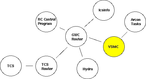
The Arcon task open a client connection to the VSMC program and send a string command that the VSMC routes through the GWC router to the different GWC clients (RC-Spectrograph Control Program, TCS Router, Hydra Control Program). The result of the operation is then sent back to the Arcon task. In such a way Arcon is now capable of communicating with many devices and still appear to have a single SMC to talk to.
back to top [55]
The Arcon API to talk to the VSMC (and to talk to any other SMC) lives in /xp/iraf/arcon/lib/motors/Drivers. It consists of several files that implement the SMC communication protocol over different communication channels. The current incarnation of the API includes support for communication through serial ports, TCL/DP channels, TCP sockets and RPC.
Selection of protocol is made by setting the "protocol" environment variable in the instrument_taks.cl file specific to each instrument. For the RC-Spectrograph the instrument_tasks.cl file lives at /xp/iraf/arcon/hardware/ctio/instruments/cs4m and the environment variable is called "lsi_protocol". This variable has to be set to "tcldp" to talk with the virtual SMC. The "lsi_host" variable must be set to the machine in which the VSMC program is running and the "lsi_port" variable has to be set to the port in which the VSMC is listening for connections that is port 2002.
back to top [55]
The VSMC software code lives at /xp/source/sun/vsmc. The structure of the directory tree is as follows:
vsmc
bin
doc
lib
bitmaps
vsmc
share
include
lib
src
api
gwcwish
The VSMC software consist of an extended TCL/TK interpreter plus a set of TCL/TK scripts that build the functionality required by the application. The extended TCL/TK interpreter lives at sub directory "src/gwcwish". Support is provided for compiling the interpreter under Linux, SunOs and Solaris. The TCL/TK scripts live at sub directory lib/vsmc.
Usually the VSMC program will automatically start as part of the RC-Spectrograph setup done by the "SetFiles -a" command. The SetFiles command allows to choose the instrument in use which in turn makes Arcon execute the specific instrument_init.cl script for that instrument to launch the VSMC program. Still it is possible to launch the program manually by typing "start_vsmc" in the Iraf command line. Arcon is also in charge of shutting the program down when Arcon is closed or restarted.
The startup script will search the /xp/source/sun/vsmc/bin directory for file "vsmcrc" to set the environment before running. If not found it will look for the default version of that file at the user home directory. Following is the vsmcrc file that actually lives at /xp/source/sun/vsmc/bin
---------------------------------------------------------------
# Environment variables
# Source the mosaic environment
source /usr/local/gwc/config/mosaic.env
# Environment variable for the VSMC home directory
setenv GCLIENT_HOME /xp/source/sun/vsmc
# Home directory of the TCL/TK library
setenv TCL_LIBRARY $GCLIENT_HOME/share/lib/tcl8.0
setenv TK_LIBRARY $GCLIENT_HOME/share/lib/tk8.0
setenv TIX_LIBRARY $GCLIENT_HOME/share/lib/tix4.1
setenv DP_LIBRARY $GCLIENT_HOME/share/lib/dp4.0
# The MPG_ROUTER variable designates the name of the host in which
# the router run. When not defined the the mpg router is supposed
# to be running in indus.tuc.noao.edu.
# Here commented out to use the definition in mosaic.env
#setenv MPG_ROUTER ctioa1
# The variable MPG_ROUTER_PORT designates the port in which the mpg
# router is listening for incoming connections. The default value
# for this variable is 1 plus the the wiyn router port (2345).
# Here commented out to use the definition in mosaic.env
#setenv MPG_ROUTER_PORT 2347
# This tell the program where to find the binaries and configurations file.
setenv GCLIENT_BIN $GCLIENT_HOME/bin
setenv GCLIENT_LIB $GCLIENT_HOME/lib
# Make sure that guidebin is in the search path
set path = ( $GCLIENT_BIN $path )
# Make sure we have the right man path
if ($?MANPATH) then
setenv MANPATH {$MANPATH}:$GCLIENT_HOME/man
else
setenv MANPATH {/usr/man}:$GCLIENT_HOME/man
endif
# Uncomment this line if running in SunOs environment
setenv LD_LIBRARY_PATH /usr/lib:/usr/local/X11R5/lib:/usr/openwin/lib
---------------------------------------------------------------
back to top [55]
The graphic user interface of the VSMC program allows the user to check for resent requests and their result as well as for the current status of the communication link to the GWC router.
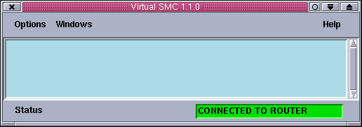
When the application starts it opens a connection to the GWC router. Then it publish some GWC command variables. Incoming Arcon request are logged into the logging panel along with a time stamp and a correlative number.
The menu bar has three menus: Options, Windows and Help.

Use the options menu to activate/deactivate the alarm bell and to quit the application. When selected the alarm bell flag activates an audible tone to signal that the communication link to the GWC router is broken.

Use the windows menu to pop up the console window and the comparison lamps interface.
back to top [55]
Use the console window to type string commands to control the RC-Spectrograph, the comparison lamps and the rotator mirror. The only command available is rcspec. The available subcommands and arguments are listed below.
rcspec all
return the current status of the RC-Spectrograph plus other devices. The order of the fields is as follows: complamp, rotator mirror, comparison lens, slit width, decker, grating tilt, collimator focus, upper filter position, lower filter position, mask position, sky suppresser position, rear slit viewer
rcspec colfocus [move|position|status|stop] value
Interface to the collimator focus mechanism.
rcspec clamp move [on|off]
Turn the old comparison lamps on or off.
rcspec complamp [move [etalon|tha|qua|hene|pen|off|park] | position | status | stop]
Command interface to the hydra comparison lamps system.
rcspec complens [move|position|status|stop] value
Command interface to the comparison lens mechanism.
rcspec lfilter [move|position|status|stop] value
Command interface to the lower filter.
rcspec mask [move|position|status|stop] value
Command interface to the newall mask mechanism.
rcspec rotatormirror [move|position|status|stop] value
Command interface to the rotator mirror.
rcspec slitwidth [move|position|status|stop] value
Command interface to the slit width mechanism.
rcspec tilt [move|position|status|stop] value
Command interface to the grating tilt mechanism.
rcspec ufilter [move|position|status|stop] value
Command interface to the upper filter mechanism.
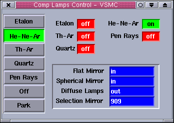
The lamps window allows the user to turn the comparison lamps system on/off and to select the comparison lamps sources.
When no motion is sensed, the status labels are blue and white. When a mechanism is active or moving the status labels blink and the background color goes yellow to reflect the new status. If no status information is available or an error condition is sensed the status labels blink and the background goes red.
back to top [55]
The logging area shows all the incoming requests to the VSMC and the exceptions that have occurred during the session. All messages are prefixed with a time stamp and a correlative number. Use the scroll bar to move across the log messages.
The status bar presents the current status of the communication link to the GWC router. When the link is broken the status label will go red and will start blinking signaling that the communication has been lost. After that, the program will start a reconnection sequence trying to connect every ten seconds to the GWC router.
"ERROR: generic client can't connect to GWC ROUTER..." - Check that the GWC router is actually running on its host machine.
If its running check that the machine in which the VSMC is running is an enabled machine. Check the /usr/local/gwc/config/routersetup.tcl file for your machine name. If not present add the name using the rest of the file as a template.
Check also that the environment variables MPG_ROUTER and MPG_ROUTER_PORT are set to the proper values in the vsmcrc file.
"WARNING: generic client not connected to GWC ROUTER..." - This warning message appears to warn the user he chose not to
connect to the GWC router.
"ERROR: illegal command: rcspec ..." - You type an unknown command. Check the list of legal commands above in this document.
back to top [55]
Last Updated: March 5, 2001
rcantaruttiATnoao.edu
| Contents: | |
| 1. | Architecture [55] |
| 2. | IcsInfo Software [55] |
ICS Info (Rev 1.0 March 2001)
Arcon requires set up information from the instrument to fill the image headers produced with each Arcon exposure. To get the header information Arcon reads the appropriate header file generated by a GWC router client called icsInfo. Icsinfo is a configurable header information server that collects the header data from different sources through the GWC router and writes it down to a file which is read by Arcon at the end of every exposure. The picture below illustrates this architecture.
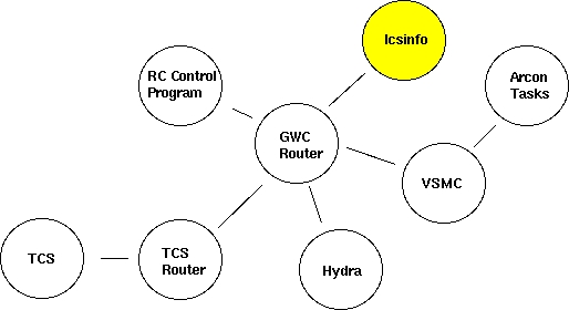
back to top [55]
The icsInfo is a TCL script that starts up automatically at Arcon boot time. The script runs forever waiting for Arcon requests to write down a header information file in the /tmp directory. The information included in that file depends on configuration files specific for each instrument.
The icsInfo source code lives at /a1xp/source/sun/icsInfo directory. The directory structure is as follows:
The icsInfo software consist of an extended TCL interpreter that runs a single TCL script. The extended TCL interpreter lives at directory icsInfo. Support is provided for compiling the interpreter under SunOs only. The TCL script lives at directory icsInfo as well.
Usually the icsInfo program starts automatically as part of the Arcon configuration set up of the instrument. The program is launched from the instrumet_init.cl Iraf script. Still it is possible to start the program manually by typing start_cs4m_info (RC-Spectrograph) at the Iraf command line.
The program will then look for the configuration files specific to the instrument in the icsInfo/Config/cs4m (RC-Spectrograph) directory. The configuration files are headers.conf and telem.conf. The file headers.conf lists the different GWC variables that icsInfo will subscribe to in order to receive header information of the instrument. The file telem.conf defines the appearance of the header file to be generated (keyword name, comments and position)
Once running the program it will present a prompt at which the user can type TCL commands. A very useful command is "fillheader". This command will dump to the screen the header file including the most resent data available.
Note: Replace the word cs4m with the arcon name of the instrument you are using. For example if you are using hydra the start up command will be start_hydra_info and the configurations files will be at icsInfo/Config/hydra.
back to top [55]
Last Updated: March 5, 2001
rcantaruttiATnoao.edu
The R-C grating spectrograph is used at the f/7.8 R-C focus of the 4.0-meter telescope where the scale is 6.56 arcsec/mm. It is identical to the one at Kitt Peak National Observatory, in construction and as far as possible, in operation. The distinguishing feature of these 4.0-meter spectrographs is their large beam size. As a result, higher dispersion than usual for Cassegrain spectrographs is available, along with excellent spatial resolution for observations of extended objects. All functions of the spectrograph can be controlled remotely by the data acquisition computer, permitting convenient and efficient operation.
In normal operation, slit viewing is accomplished by means of a TV mounted on the instrument rotator. Two positions of the instrument rotator mirror carriage provide for direct viewing of the field, for target acquisition and for viewing light reflected from the spectrograph slit. The field of view in slit viewing mode is somewhat restricted, so that only the central arc minute of the spectrograph slit is visible on the TV. Auto guiding is normally accomplished using a separate TV camera, optically coupled to the offset guide probe, mounted in the instrument rotator, in conjunction with a leaky guider module. It is also possible to connect the same leaky guider to the slit viewing TV in order to permit auto guiding on light reflected from the slit jaws. Full details of the acquisition TV system and auto-guiders can be found in Section III. The spectrograph itself has both front-slit and rear-slit viewing optics.
The spectrograph may be rotated by up to 180 under remote control from the console room, with the telescope in any position. Observer support personnel should be notified of your intention to do so at the start of your run so that they can ensure that all cables have been routed to permit this. Normally the spectrograph is mounted with the slit E-W (PA=90 ).
The optical diagram for the spectrograph is given in Figure IV-1. The following descriptive sections are listed in the order which light passes through the spectrograph.
The decker plate for defining the length of the slit has five stellar/comparison pairs, a pointer for marking the center of the slit, a position for holding a calibration wedge, and a fully open position. The relevant dimensions are listed in Table IV-1.
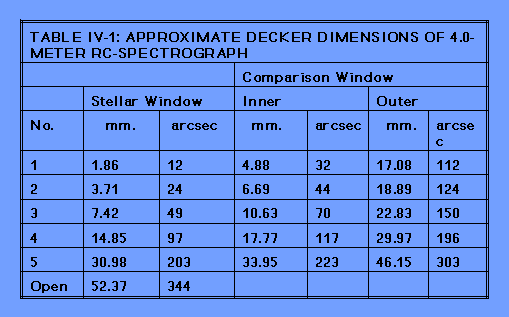
The entrance slit has a length of 50 mm. Its width has a range from closure to 50 mm. One second of arc corresponds to approximately 150 microns. The size of the slit projected on the detector can be calculated from the information given in Figure IV-2. The conventional slit can be replaced by an aperture plate, permitting the acquisition of spectra of several objects distributed over an approximately 5 arcmin diameter field. Aperture plates are currently prepared in advance at NOAO Tucson. A TV camera can be attached to the rear-slit viewing periscope to assist in registering the apertures with the program objects. Observers with a potential interest in this system should contact CTIO staff well in advance of their run.
The multiple aperture plate contains 55 holes each 150 wide (1 arcsec) at 1.0 mm (6.6 arcsec) intervals along the slit. Exposures of the quartz lamp or white spot taken through these multi-holes are used to calibrate the geometric distortions introduced by the detector/camera combination for long slit work.
Two filter bolts are available each containing four filters plus a clear position. The lower filter bolt always contains neutral density filters; the upper-filter bolt either contains further neutral density filters or order sorting filters. An additional holder to contain a single order sorting filter can be manually placed in the beam if required. Note that this can only be done with the image tubes turned off if the 2D-Frutti is in use. Since all these filters are below the slit, the appropriate filters should be in place when the spectro- graph is focussed. The available filters are listed in Table IV-2.
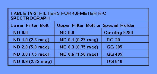
A four-position plate acts as a shutter and Newall mask. The positions are: open, closed, mask north half and mask south half. The latter two are used for quantitative focusing of the spectrograph. Successive exposures of a comparison source are taken through each mask. At perfect focus, the positions of the arc lines in these exposures coincide exactly. Increasing departures from focus lead to greater displacements between the images. An additional high speed computer controlled shutter is used to obtain precisely timed exposures.
The collimator mirror is an off-axis paraboloid of 225 mm diameter and 1161 mm focal length. The point-source beam size is 152 mm. The collimator has a travel of 38.1 mm for focusing the image of the slit onto the detector.
At present, there are thirteen 203 by 254 mm gratings available. Their nominal specifications are listed in the Table IV-3. Table IV-4 lists the resolution and coverage available with various detectors. Tables IV- 5, IV-6, and IV-7 list grating efficiencies.
Two Air Schmidt cameras are available. The Air Schmidt camera is a field-flattened Schmidt camera of 229 mm focal length and 229 mm clear aperture. This camera is exclusively used with a CCD detector, which together with its special dewar, forms an integral part of the camera. All optical surfaces of the "red" Air Schmidt are coated to give optimal performance in the red and as a result, this camera cannot be used blueward of 4500 , the "blue" Air Schmidt can be used at all optical wavelengths (3000 - 10000 ) but is less efficient that the "red" Air Schmidt redward of 5000 .
The Folded Schmidt camera is also a field-flattened Schmidt camera with 229 mm focal length and optical characteristics almost identical to the Air Schmidt. The corrector is optimized for blue and near UV wavelengths. The incorporation of a folding flat in the optical train brings the focal plane outside the body of the camera, permitting its use with the 2D-Frutti photon counting system or the CCDs mounted in standard "direct" dewars. This causes the camera to have somewhat less clear aperture and consequently greater vignetting than the Air Schmidt. On-axis, the Folded Schmidt has nearly the same throughput as the Air Schmidt. For distances of greater than 10 mm off-axis, the through-put begins to fall off significantly. The uv transmitting optics provide for excellent throughput at wavelengths all the way down to the atmospheric cutoff.
Two calibration sources, Th-Ar and He-Ne-Ar, are mounted in the instrument rotator. It is possible to turn on the He-Ar and the Ne lamps separately. A quartz continuum lamp for flat-field calibration is also available. With a manually operated filter bolt in the rotator, it is possible to attenuate the comparison source light by a factor of either three or ten. A lens is moved over the slit of the spectrograph to provide an f/7.6 beam for comparison exposures.
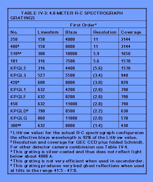
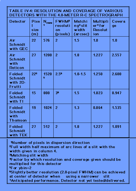
Links
[1] http://www.ctio.noao.edu/noao/sites/default/files/instruments/spectrographs/4mRC-optics.gif
[2] http://www.ctio.noao.edu/noao/content/acquisition-guiding-f8-focus
[3] http://www.ctio.noao.edu/noao/content/Filters-use-4m-R-C-SPec
[4] http://www.ctio.noao.edu/noao/sites/default/files/instruments/filters/anamorph.gif
[5] http://www.ctio.noao.edu/noao/sites/default/files/instruments/filters/g250.gif
[6] http://www.ctio.noao.edu/noao/sites/default/files/instruments/filters/g400.gif
[7] http://www.ctio.noao.edu/noao/content/loral-3k-arcon35-4m-r-c-spectrograph
[8] http://www.ctio.noao.edu/noao/sites/default/files/instruments/filters/qe.gif
[9] http://www.ctio.noao.edu/noao/content/SlitDecker
[10] http://www.ctio.noao.edu/noao/sites/default/files/instruments/spectrographs/HeAr_low_3800to7200.gif
[11] http://www.ctio.noao.edu/noao/sites/default/files/instruments/spectrographs/HeAr_low_3800to7200.pdf
[12] http://www.ctio.noao.edu/noao/sites/default/files/instruments/spectrographs/HeAr_med_3000to4100.gif
[13] http://www.ctio.noao.edu/noao/sites/default/files/instruments/spectrographs/HeAr_med_3000to4100.pdf
[14] http://www.ctio.noao.edu/noao/sites/default/files/instruments/spectrographs/HeAr_med_3800to5250.gif
[15] http://www.ctio.noao.edu/noao/sites/default/files/instruments/spectrographs/HeAr_med_3800to5250.pdf
[16] http://www.ctio.noao.edu/noao/sites/default/files/instruments/spectrographs/HeAr_high_4240to4620.gif
[17] http://www.ctio.noao.edu/noao/sites/default/files/instruments/spectrographs/HeAr_high_4240to4620.pdf
[18] http://www.ctio.noao.edu/noao/sites/default/files/instruments/spectrographs/HeNeAr_low_4900to9700.gif
[19] http://www.ctio.noao.edu/noao/sites/default/files/instruments/spectrographs/HeNeAr_low_4900to9700.pdf
[20] http://www.ctio.noao.edu/noao/sites/default/files/instruments/spectrographs/HeNeAr_med_5300to7000.gif
[21] http://www.ctio.noao.edu/noao/sites/default/files/instruments/spectrographs/HeNeAr_med_5300to7000.pdf
[22] http://www.ctio.noao.edu/noao/sites/default/files/instruments/spectrographs/HeNeAr_med_6700to8300.gif
[23] http://www.ctio.noao.edu/noao/sites/default/files/instruments/spectrographs/HeNeAr_med_6700to8300.pdf
[24] http://www.ctio.noao.edu/noao/sites/default/files/instruments/spectrographs/HeNeAr_med_8200to9800.gif
[25] http://www.ctio.noao.edu/noao/sites/default/files/instruments/spectrographs/HeNeAr_med_8200to9800.pdf
[26] http://www.ctio.noao.edu/noao/content/instrument-control-software-blanco-rc-spectrograph
[27] http://www.ctio.noao.edu/noao/content/4mrc-virtual-smart-motor-controller
[28] http://www.ctio.noao.edu/noao/content/4mrc-ics-info
[29] http://www.ctio.noao.edu/noao/content/4m-rc-basic-optical-characteristics
[30] http://www.ctio.noao.edu/noao/sites/default/files/instruments/spectrographs/control_panelp.gif
[31] http://www.ctio.noao.edu/noao/sites/default/files/instruments/spectrographs/grating_setupp.gif
[32] http://www.ctio.noao.edu/noao/sites/default/files/instruments/spectrographs/extract%20positionp.gif
[33] http://www.ctio.noao.edu/noao/sites/default/files/instruments/spectrographs/enable_rc_motorp.gif
[34] http://www.ctio.noao.edu/noao/sites/default/files/instruments/spectrographs/initializep.gif
[35] http://www.ctio.noao.edu/noao/sites/default/files/instruments/spectrographs/Writer_rc_parameterp.gif
[36] http://www.ctio.noao.edu/noao/sites/default/files/instruments/spectrographs/sv14114142.jpg
[37] http://www.ctio.noao.edu/noao/sites/default/files/instruments/spectrographs/sv14114151.jpg
[38] http://www.ctio.noao.edu/noao/sites/default/files/instruments/spectrographs/sv14114149.jpg
[39] http://www.ctio.noao.edu/noao/sites/default/files/instruments/spectrographs/sv14114146.jpg
[40] http://www.ctio.noao.edu/noao/sites/default/files/instruments/spectrographs/sv14114153.jpg
[41] http://www.ctio.noao.edu/noao/sites/default/files/instruments/spectrographs/sv14114155.jpg
[42] http://www.ctio.noao.edu/noao/sites/default/files/instruments/spectrographs/sv14114159.jpg
[43] http://www.ctio.noao.edu/noao/sites/default/files/instruments/spectrographs/sv14114163.jpg
[44] http://www.ctio.noao.edu/noao/sites/default/files/instruments/spectrographs/sv14114165.jpg
[45] http://www.ctio.noao.edu/noao/sites/default/files/instruments/spectrographs/sv14114167.jpg
[46] http://www.ctio.noao.edu/noao/sites/default/files/instruments/spectrographs/sv14114169.jpg
[47] http://www.ctio.noao.edu/noao/sites/default/files/instruments/spectrographs/sv14114171.jpg
[48] http://www.ctio.noao.edu/noao/sites/default/files/instruments/spectrographs/sv14114173.jpg
[49] http://www.ctio.noao.edu/noao/sites/default/files/instruments/spectrographs/sv14114179.jpg
[50] http://www.ctio.noao.edu/noao/sites/default/files/instruments/spectrographs/sv14114181.jpg
[51] http://www.ctio.noao.edu/noao/sites/default/files/instruments/spectrographs/sv14114189.jpg
[52] http://www.ctio.noao.edu/noao/sites/default/files/instruments/spectrographs/sv14114183.jpg
[53] http://www.ctio.noao.edu/noao/sites/default/files/instruments/spectrographs/sv14114185.jpg
[54] http://www.ctio.noao.edu/noao/sites/default/files/instruments/spectrographs/sv14114187.jpg
[55] http://www.ctio.noao.edu/noao