CTIO Filters
The NOAO MOSAIC Imager II (as did the BTC before it) takes square filters 146 x 146 mm, 12 mm thick. We are slowly increasing our stock of filters in this size, so if you don't see what you need here, please contact us. What do we have, and what are the focus offsets? [1]
The SOAR Optical Imager (minimosaic of two 2Kx4K EEV CCDs) and the Schmidt use 4 inch square filters up to 10 mm thick. We have quite a selection of filters in this size, see the 3" & 4"filter list [2]. Recent acquisitions are:
For Cass imaging we use 3 inch square filters up to 10 mm thick. We have quite a good selection of filters in this size too. The cass filter wheel assembly has two wheels holding up to 8 3x3 filters each. We also have a single module that can hold 5 4x4 filters, so filters in this size can be used if we don't have a 3x3 equivalent.
Now and then people have asked to use one or more of our 2x2 inch interference filters due to not having it in 3x3 or 4x4 inch size, being prepared to accept some vignetting. Be warned! Most of these filters are many years old, and some have seen a lot of use. If you want to use some weird filter it's better to (a) buy one yourself, or (b) convince us to buy it for you. Filters can take a long time to make (several months to over a year for the 146x146 mm narrow band filters). Prices vary with manufacturer, and the specifications you ask for, we can recommend if you like. Plan on spending $2500 - $5000 for a 146 x 146 mm filter, half that for 3x3 inch or 4x4 inch.
Alistair Walker 17 April 2000, updated 4 April 2006
| Contents: | |
| Description | |
| Transmission Measurement Procedure | |
| Instructions for plotting nice graphs | |
| Tricks for the measurements |
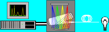
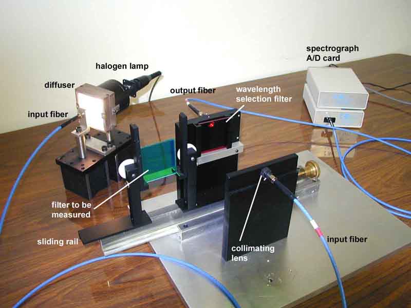
During January 2001, a new setup was assembled to measure filter transmission on Cerro Tololo . Any thickness, shape and size of filters up to 6x6" can be measured.
The S2000 is a miniature fiber optics spectrometer made by Ocean Optics [3] with grating of 600 lines/mm blazed for 750 nm, configured for spectral range of 600-1200 nm, with 10um wide slit and long pass filter (305nm) permanently installed. UV2, a UV detector upgrade for application < 360 nm, and L2, a detector collecting lens of fused silica for increased light collector efficiency, were also requested from Ocean Optics. Fiber optics with 400um core diameter are used.
The fiber optics spectrometer S2000 is a crossed Czerny-Turner design, with no moving parts. The basic characteristic of the Czerny-Turner mount is to use two identical off-axis concave spherical mirrors as the collimating and focusing elements, with the important property of canceling the coma aberration that is inherent with spherical mirrors and which otherwise inhibit resolution.
Light enters the optical fiber and is efficiently transmitted to the spectrometer. Once in the spectrometer, a spherical mirror collimates the divergent light emerging from the optical fiber. A plane grating diffracts the collimated light, the resulting diffracted light is focused by a second spherical mirror. An image of the spectrum is projected onto a 1 x 2048 linear CCD array, and the data is transferred to a computer through an A/D card.
The light source used is a halogen lamp with a quartz bulb (General Electric 787, same as the ones used for the 4m dome flat lights), that we feed with a stabilized power supply at 7V (1.77 A). A ground glass in front of the lamp is used to create a diffuse source.
The Spectrometer comes with the OOIBase32 software, which is the spectrometer operation software. From time to time it is necessary to check the calibration of the spectrometer's wavelength. For this we use a light source that produces known spectral lines, in our case Ocean Optics' HG-1 Mercury-Argon lamp. We did that calibration in Jan 2001 and found the following parameters:
which produced a maximal residual error of 0.2 nm. Follow the guideline in the help menu to perform the calibration.
 , press
  to take a spectrum of the light source, adjusting integration time (1) until you get about 3000 count maximum.
 (on first icon line), wait until you see a trace at the zero level and take a Global Dark
  (on first icon line)
 (on second icon line): you should then see a flat line at 100 % (maybe with some isolated vertical lines, if not go back to Scope mode and retry).and the absolute transmission curve should appear.
Notes:
1. The longer the integration time, the slower the system refresh time. At about 500ms, it is already noticeably slow, at 1sec integration time, it becomes terribly slow and sometimes fails. Whenever the software freezes, you need to exit the program, cycle the spectrometer power and start again.
2. In each step make sure the data is well taken by watching out the status message (should say 'Ready').
3. Use average (5 to 10) if the signal is noisy. References, dark and measurements must be taken under same conditions (integration, average,...)
For data processing we recommend to use Microcal Origin Software. This software has useful functions (like smoothing and Gaussian Fit that Excel doesn't have as readily).
* Import the file saved by OOIBase to an Origin worksheet. Select File | Import | ASCII select the *.* extension.
* Plot the data: Plot and select the type of plot you want. We suggest 'Line'.
* Choose your column variables for the X and Y axes.
* You can re-scale the Graph by clicking the axes or choosing Graph.
* You can always add new columns in the table selecting the Columns menu. Handling the columns of numbers is very similar to what is done with Excel.
For some plots it will be useful to use the "Smoothing" or "Fit as Gaussian" options. For Smoothing activate the Graph and select: Analysis | Smoothing | Adjacent Averaging. This opens the Smooth Points dialog box were you specify the variable that control the degree of smoothing. The smoothed value at index i is the average of data points in the interval [i-(n-1)/2 , i + (n-1)/2]. Increase the degree of smoothing until you get satisfactory results (20 is usually enough). Then plot again choosing as new variable the smoothed column.
To fit Gaussian select Analysis | Fit Gaussian. That function is useful especially for narrow band filters to avoid the triangular peak that usually shows up because of the finite resolution. Make sure the fit is good, ie. the peak, Fwhm and slopes are not affected in the process.
Worksheet and graph may be exported to another applications by creating an export file. Activate the data table and select File | Export ASCII. If you want to export the Graph, select File | Export Page and choose the file type you want to export.
To save select File | Save Project As
In all measurements, you need a wavelength selection filter to separate the orders. In general we use two selection filters: Corion short wave pass LS 550 (plot [4] and data [5]) and Schott long wave pass OG 590 [6].
* For all filters with transmission range above 590 nm, you will see the transmission in first order directly and need to use OG 590.
* For all filters with transmission range below 550 nm, you will see the transmission in second order and need to use LS 550 (and divide the wavelength obtained by two).
* For all filters with transmission range around 550-590 nm, you need to make 2 sets of data, one with the LS600 selection filter and possibly one with the OG590 selection filter, then stitch together the results to obtain a single graph. Usually the resulting graph has some noise at the union, so you need to smooth it.
* For blue filters, you might want to use the Bj filter for better transmission (less noise at 3300 A).
* For measurements near the atmospheric cutoff at 330nm, use the UVpass Corion filter (see plot [7])
Measuring a filter against itself will show you a line at 100% in the useful transmission range of the filter and increasing noise outside that range, which is sometimes useful to assess the bandpass width of the filter in order to select the most appropriate wavelength selection filter for the absolute transmission measurement.
See the filters [8] already remeasured with this new setup.
Written by Constanza Araujo (optics student at the Catholic University of Vaparaiso), 1 February 2001.
The standard filter size for the 0.9-m and 1.5-m CFCCD is 3x3 inch, which are mounted in two filter wheels which each can hold up to 8 filters (or 7 plus clear). We have a single wheel which can hold up to 5 4x4 inch filters which can be installed in place of one of the 8-position wheels. At the Schmidt, and the 4-m PFCCD (now retired) 4x4 inch filters are required in order to avoid vignetting. We do have adaptors to allow the use of smaller filters (eg 2x2 inch), if the vignetting is tolerable, but see the warning note at the head of the filter list. The BTC and Mosaic II imagers, used at the 4-m prime focus, take filters 5.75 x 5.75 inches (146x146 mm) and nominally 12 mm thick.
| FILTER | SIZE | Thick | Cent | fwhm | Trans | FILTER SET | Filter curves | COMMENTS | |
| /width | (") | (mm.) | (A) | (A) | (%) | Plot |
Data file |
||
| 3513/628 | 4X4 | SDSS u | |||||||
| 3530/280 | 4x4 | 9.15 | 3530 | 280 | 37.14 | u Stromgren | |||
| 3570/660 | 3x3 | 3570 | 660 | 80.59 | U liq. CuSO4 Tek set #2 | ||||
| 3575/600 | 3x3 | 9.09 | 3575 | 600 | 74.21 | U liq. CuSO4 Tek set #1 | |||
| 3580/610 | 4x4 | 9.32 | 3580 | 610 | 74.66 | U liq. CuSO4 set#1 4mts | |||
| 36237605 | 3x3 | 8.83 | 3623 | 605 | 67.66 | U liq. CuSO4 Tek set#3 | |||
| 3960/100 | 4x4 | Ca H&K line filter | |||||||
| 3996/1042 | 3x3 | 8.11 | 3996 | 1042 | 62.70 | C Wash | |||
| 4000/1030 | 4x4 | 8.45 | 4000 | 1030 | 62.45 | C Wash | |||
| 4118/146 | 4x4 | 9.87 | 4118 | 146 | 52.04 | v Stromgren 4x4 | |||
| 4185/1030 | 4x4 | 5.40 | 4185 | 1030 | 70.44 | B Harris set#1 4mts | |||
| 4202/1050 | 3x3 | 4200 | 1050 | 66.16 | B Tek set#2 | ||||
| 4203/1050 | 3x3 | 5.26 | 4200 | 1050 | 66.72 | B Tek set#3 | |||
| 4201/1050 | 3x3 | 5.17 | 4200 | 1050 | 66.48 | B Tek set#1 | |||
| 4340/980 | 3x3 | 6.38 | 4341 | 980 | 60.33 | B Harris set 1 | |||
| 4357/1665 | 4x4 | 3.65 | 4357 | 1665 | 88.19 | B Tyson "J" | |||
| 4345/980 | 3x3 | 6.33 | 4345 | 980 | 60.85 | B Harris set 2 | |||
| 4200/1050 | 4x4 | B set# 2 Schmidt | |||||||
| 4697/196 | 4x4 | 9.85 | 4697 | 196 | 71.27 | b Str"m. 4x4 | |||
| 4759/1430 | 4x4 | SDSS g | |||||||
| 4940/700 | 4x4 | 8.95 | 4920 | 670 | 93.09 | Gunn g | |||
| 5025/1023 | 3x3 | 8.08 | 5025 | 1023 | 88.60 | M Wash. | |||
| 5019/50 | 4x4 | 7.83 | 5027 | 50 | 79.48 | ||||
| 5040/990 | 4x4 | 8.25 | 5040 | 990 | 88.23 | M Wash. | |||
| 5118/900 | 3x3 | 5.05 | 5118 | 900 | 81.39 | g Gunn-T | |||
| 5130/155 | 4x4 | 7.76 | 5121 | 133 | 84.13 | DDO 51 Wash. set | |||
| 5295/1590 | 4x4 | 5.24 | 5292 | 1625 | 90.66 | HST "V" | |||
| 5362/895 | 3x3 | 6.14 | 5362 | 895 | 76.80 | V Harris set 1 | |||
| 5370/900 | 3x3 | 6.18 | 5370 | 900 | 75.64 | V Harris set 2 | |||
| 5438/1026 | 3x3 | 5438 | 1026 | 91.91 | V Tek set#2 | ||||
| 5443/1060 | 4x4 | V set#2 Schmidt | |||||||
| 5443/1060 | 4x4 | 5.12 | 5443 | 1060 | 88.50 | V Harris set#1 4mts | |||
| 5475/1000 | 3x3 | 5475 | 1000 | 87.71 | V Tek set #1 | ||||
| 5497/241 | 4x4 | 9.74 | 5478 | 244 | 70.83 | y Str"m. 4x4 | |||
| 6120/140 | 3x3 | 7.97 | 6115 | 135 | 85.89 | Supernova | |||
| 6130/590 | 4x4 | 8.35 | 6130 | 590 | 56.19 | T1 Wash. | .9% leak at 1.2u. | ||
| 6152/625 | 3x3 | 8.21 | 6152 | 625 | 58.06 | T1 Wash. | 1% leak at 1.0u. | ||
| 6265/1483 | 4x4 | SDSS r | |||||||
| 6410/1470 | 3x3 | 5.23 | 6410 | 1470 | 81.76 | R Tek set#3 | |||
| 642571500 | 3x3 | 5.25 | 6425 | 1500 | 79.69 | R Tek set#1 | |||
| 6437/1525 | 4x4 | 5.22 | 6437 | 1525 | 81.38 | R harris set#1 4mts | |||
| 6437/1525 | 4x4 | R set #2 Schmidt | |||||||
| 6400/1450 | 3x3 | 6400 | 1450 | 81.09 | R Tek set #2 | ||||
| 6475/1600 | 3x3 | 6.18 | 6475 | 1600 | 81.70 | R Harris set 1 | |||
| 6493/1445 | 3x3 | 6.15 | 6493 | 1445 | 77.00 | R Harris set 2 | |||
| 6560/900 | 4x4 | 9.19 | 6495 | 900 | 94.95 | Gunn r | |||
| 656375-3 | 3x3 | 5.61 | 6559 | 64 | 89.37 | ||||
| 656375-4 | 4x4 | 5.54 | 6567 | 68 | 82.32 | ||||
| 660075-3 | 3x3 | 5.57 | 6598 | 69 | 87.77 | ||||
| 660075-4 | 4x4 | 5.57 | 6600 | 67 | 84.77 | ||||
| 6728/1000 | 3x3 | 5.05 | 6728 | 1000 | 93.83 | r Gunn-T | |||
| 6738/50 | 4x4 | 7.97 | 6744 | 50 | 87.83 | ||||
| 7734/50 | 4x4 | SDSS i | |||||||
| 8120/1500 | 4x4 | 9.22 | 8065 | 1600 | 86.60 | Gunn i | |||
| 8067/1485 | 3x3 | 6.11 | 8067 | 1485 | 95.49 | I kc Tek set#3 | |||
| 8075/1500 | 3x3 | 6.13 | 8075 | 1500 | 95.53 | I kc Tek set#1 | |||
| 8075/1500 | 4x4 | 6.19 | 8075 | 1500 | 94.09 | I kc set#1 4mts | |||
| 8118/1415 | 3X3 | 8118 | 1415 | 96.63 | I kc Tek set#2 | ||||
| 8100/1500 | 3X3 | 5.08 | 8100 | 1500 | 93.00 | I Gunn-T | |||
| 8300/2500 | 4x4 | 5.43 | 8310 | 2560 | 98.73 | HST "I" | |||
| 9100/1400 | 4x4 | SDSS z | |||||||
| 9100/1400 | 4x4 | z Gunn | |||||||
| 9100/1400 | 3x3 | z Gunn | |||||||
ISPI is offered with the broad band Y, J, H, Ks filters, as well as a set of narrow band filters. Basic data are given in the tables below. Filter scans are available for some of the filters here [9].
| Filter |
Central wavelength (micron) |
Wavelengths @80% (micron) |
|
|---|---|---|---|
| J | 1.25 | 1.176 | 1.322 |
| H | 1.635 | 1.5005 | 1.7705 |
| Ks | 2.150 | 1.9915 | 2.2955 |
| Y | 1.0381 | BW 0.1457mu | |
Fluxes, isophotal wavelengths, and isophotal frequencies for Vega have been determined by Tokunaga and Vacca [10] for J, H, and K' filters which comprise part of the MKO/Gemini filter set. Copies of these filters were used in ISPI up until 2004B.
| Filter |
Central wavelength (micron) |
Wavelengths @80% (micron) |
|
|---|---|---|---|
| Cont-203 | 2.0336 | 2.0262 | 2.0400 |
| He I | 2.0618 | 2.0545 | 2.0674 |
| C IV | 2.0826 | 2.0753 | 2.0892 |
| H2 | 2.1262 | 2.125 | 2.146 |
|
Continuum, 2.14 mu |
2.1462 | 2.1385 | 2.1532 |
| Br gamma | 2.1648 | 2.1592 | 2.1738 |
| He II | 2.1911 | 2.1845 | 2.1976 |
| H2 & continuum 2.25 mu | 2.2527 | 2.2428 | 2.2618 |
February 12, 2007
A. Walker 18 Dec 2002
The Mosaic II imager, used at the Blanco 4-m prime focus, takes filters that are 146x146mm and 12mm (nominal) thick.
Focus offsets are referred to the R filter, since this is the filter we use for taking focus frames each night when the Mosaic is installed in order to monitor telescope performance.
We are (slowly) measuring these filters, let us know if there is any one you particular want to have us scan. Note that the Sloan set (griz) and the Johnson-Cousins BVR (but not I) sets should be near-identical to those at KPNO, see the KPNO Mosaic Filters. [11]
A set of standardized filter names and IDs have been developed to ensure proper application of astrometric solutions and real-time display processing (as well as future archive uniformity). These official names are listed in the Mosaic filter list [12]web page.
| Filter |
Center wavelegth |
fwhm |
focus offset microns |
NOAO code |
Status |
| U | 3570 | 650 | -185 | c6001 | OK |
| B | 4360 | 990 | +10 | c6002 | OK |
| V | 5370 | 940 | +30 | c6026 | from 21 OCT 2000 |
| R | 6440 | 1510 | 0 | c6004 | OK ... filter offset ref |
| I | 8050 | 1500 | +10 | c6028 | from 24 May 2003 |
|
VR Stubbs aka VR Supermacho |
6100 | 2000 | 0 | c6027 | transmission curve [13] |
| C (Wash) | 4000 | 1000 | +260 | c6006 | OK |
| M (Wash) | 5020 | 1020 | +260 | c6007 | OK |
| D51 (DDO) | 5130 | 154 | -55 | c6008 | OK |
| [OII] | 3727* | 50 | ? | c3012 | not tested yet |
| [OIII] | 4990* | 60 | +130 | c6014 | OK |
| Halpha | 6563* | 80 | +65 | c6009 | cwl, fwhm nominal |
| Halpha+8 | 6650* | 80 | -35 | c6011 | cwl, fwhm nominal |
| [SII] | 6725* | 80 | +60 | c6013 | cwl, fwhm nominal |
| u (SDSS) | 3600 | 400 | +230 | c6021 |
cwl, fwhm approx, Red Leak! [14] |
| g (SDSS) | 4813 | 1537 | +30 | c6017 |
"set #2" (in use 8/2000-) |
| r (SDSS) | 6287 | 1468 | +120 | c6018 |
"set #2" in use 8/2000-) |
| i (SDSS) | 7732 | 1548 | -20 | c6019 |
"set #2" (in use 8/2000-) |
| z (SDSS) | 9400 | 2000 | -15 | c6020 | OK |
| Bj (Tyson) | 4350 | 1650 | ? | c6024 |
#3, on loan from A. Tyson |
| I (Tyson) | 8800 | 2000 | ? | c6025 | cwl, fwhm approx |
| White | 6500 | 5000 | ? | c6016 |
just a piece of fused silica |
|
|
|||||
| Retired Filters | |||||
| g (SDSS) | 4825 | 1380 | ? | c6015 |
"set #3", red cut-off a bit too red (in use <8/2000) |
| V | 5370 | 940 | 115 | c6003 |
small chip in corner, in use <10/2000 |
| Bj | 4350 | 1650 | ? | -- | broken... |
| Bj | 4350 | 1650 | ? | -- | broken... |
| I | 8050 | 1500 | +25 | c6005 |
Filter damaged Nov 2002- The are civered by CCD-1 (SW corner) is unusable |
* = NOTE that the central wavelength of narrow band filters (actually all filters, but it is only significant for narrow band filters) is shifted aprox. 15A to the BLUE in the f/2.87 beam of the Blanco 4m + PFADC corrector as compared to the transmission measured in parallel light. The central wavelengths quoted above are nominally for when the filters are used at PF, with the aprox. 15A shift included.
Last updated: 2003 June 4 by C.Smith
Staff Contacts:
Alistair Walker: awalkerATnoao.edu
Chris Smith: csmithATnoao.edu
Subject: There is a leak -- just how much does it matter -- your call
Date: Fri, 8 Mar 2002 16:25:43 -0700 (MST)
From: Buell Jannuzi
Hi Guys,
Well there is a red leak in the ctio SDSS u' filter -- at a very low level, but perhaps enough to explain the flat field counts Mauro reports -- I'm afraid I have not had time to think this through carefully. Below are attached the asci data files containing the traces (done in the center of the filter) made by Jim DeVeny. The good news is that in the band-pass the ctio SDSS u' filter is a good match to the tracing I have on file for the actual SDSS u' filter (measured in air -- not in vacuum as actually used). The bad news is that while the SDSS u' does not appear to have a red leak (actual measurements of that filter between 8100 and 1100 angstroms so nothing), apparently because in addition to the 1mm UG11 + 1mm BG38 there is a film to, and now I'm quoting the message I got in 1996 about this filter, "suppresses a strong leak around 7000 Angstroms and acts as an AR coating in the passband. Now, the ctio SDSS u' filter does not have strong leak at 7000 -- but does have a leak near H-alpha (0.04%, tiny), with an increasing leak longward of 8000, but again, not huge -- but very significantly different from the SDSS filter.
As I said, I'm not 100% sure the measured leak accounts for Mauro's measured count difference in the flats he took last night -- but given the tracing I'm hard pressed to understand how the ctio SDSS u' filter could yield more counts than the Harris U without there being a significant leak (one might have hoped that the poor red response of the CCDs might have helped, but it looks like they are hot enough in the red to see some of the leaked light).
Buell
Attached files:
Note that the two data files will differ ever so slightly in the region covered by both tracings, but the slit used was 5 times larger (lower res) in the second set up.
The Mosaic II imager, used at the Blanco 4-m prime focus, takes filters that are 146x146 mm and 12 mm (nominal) thick. A set of standardized filter names and IDs for both Mosaic I on the KPNO Mayall and Mosaic II on the CTIO Blanco have been developed to ensure proper application of astrometric solutions and real-time display processing (as well as future archive uniformity). These official names are listed in the Mosaic filter list [12] web page.
Focus offsets are referred to the R filter, since this is the filter we use for taking focus frames each night when the Mosaic is installed in order to monitor telescope performance.
Note that the Sloan set (griz) and the Johnson-Cousins BVR (but not I) sets should be near-identical to those at KPNO, see the KPNO Mosaic Filters [11].
Note: The central wavelength of narrow band filters (actually all filters, but it is very significant for narrow band filters) is shifted approx. 15A to the BLUE in the f/2.87 beam of the Blanco 4m + PFADC corrector as compared to the transmission measured in parallel light. The central wavelengths quoated below are nominally for when the filters used at PF, with the approx. 15A shift included. Furthermore, the filter transmission curves presented below show the simulated filter tranmission curve for the Blanco 4m + PFADC f/2.87 beam.
Note: The Blanco prime focus corrector has poor response in the UV: 90% (4000A), 85% (3800A), 74% (3650A), 54% (3500A), 31% (3400A), 11% (3350A), 0% (3300A). These are calculations from the glass types and AR coating specifications, and the figures for 3300-3400A are rather uncertain. YOU STRONGLY ENCOURAGED TO USE THE u(SDSS) filter rather than the U filter. Neither of these filters, in combination with the CCDs and optical corrector, match the standard passbands perfectly. The U filter uses a (troublesome!) copper sulphate solution as red blocker, whereas the SDSS u filter is an interference filter.
| Filter |
Central Wavelength (A) |
FMHM (A) |
Focus Offset (um) |
Status |
NOAO Code |
Transmission Curves |
|
| Plot | Data File | ||||||
| U | 3570 | 650 | -185 | Ok | c6001 | .jpg [19] .ps [20] | . txt [21] |
| B | 4360 | 990 | +10 | OK | c6002 | .jpg [22] .ps [23] | . txt [24] |
| V | 5370 | 940 | -30 | From 21 Oct 2000 | c6026 | .jpg [25] .ps [26] | . txt [27] |
| R | 6440 | 1510 | 0 | Ok; filter offset ref | c6004 | .jpg [28] .ps [29] | .txt [30] |
| I | 8050 | 1500 | +10 | from 24 May 2003 | c6028 | .jpg [31] .ps [32] | .txt [33] |
|
VR Stubbs (aka VR Supermacho) |
6100 | 2000 | 0 | Ok | c6027 |
.jpg [34] .ps [35] old.jpg [36] |
.txt [37] |
| C (Wash) | 3850 | 1075 | +260 | from 05 Jan 2011 | c6029 | .jpg [38] .pdf [39] | |
| M (Wash) | 5115 | 1375 | +260 | Ok | c6007 | .jpg [40] .ps [41] | .txt [42] |
| D51 (DDO) | 5130 | 154 | -55 | Ok | c6008 | .jpg [43] .ps [44] | .txt [45] |
| [OII] | 3727 | 50 | ? | c6012 | .jpg [46] .ps [47] | .txt [48] | |
| [OIII] | 4990 | 50 | +130 | Ok | c6014 | .jpg [49] .ps [50] | .txt [51] |
| Halpha | 6563 | 80 | +65 | cwl, FWHM nominal | c6009 | .jpg [52] .ps [53] | .txt [54] |
| Halpha+80 | 6650 | 80 | -35 | cwl, FWHM nominal | c6011 | .jpg [55] .ps [56] | .txt [57] |
| [SII] | 6725 | 80 | +60 | cwl, FWHM nominal | c6013 | .jpg [58] .ps [59] | .txt [60] |
| u (SDSS) | 3600 | 400 | +230 |
cwl, FWHM approx, replacement for c6021, NO RED LEAK |
c6022 | .jpg [61] .ps [62] | .txt [63] |
| g (SDSS) | 4813 | 1537 | +30 | "set #2" (in use 8/2000-) | c6017 | .jpg [64] .ps [65] | .txt [66] |
| r (SDSS) | 6287 | 1468 | +120 | "set #2" (in use 8/2000-) | c6018 | .jpg [67] .ps [68] | .txt [69] |
| i (SDSS) | 7732 | 1548 | -20 | "set #2" (in use 8/2000-) | c6019 | .jpg [70] .ps [71] | .txt [72] |
| z (SDSS) | 9400 | 2000 | -15 | Ok | c6020 | .jpg [73] .ps [74] | .txt [75] |
| Bj (Tyson) | 4350 | 1650 | ? | #3, on loan from A. Tyson | c6024 | .jpg [76] .ps [77] | .txt [78] |
| I (Tyson) | 8800 | 2000 | ? | cwl, FWHM approx | c6025 | .jpg [79] .ps [80] | .txt [81] |
| White | 6500 | 5000 | Fused Silica | c6016 | |||
| Filter |
Central Wavelength (A) |
FMHM (A) |
Focus Offset (um) |
Status |
NOAO Code |
Transmission Curves | |
| Plot | Data File | ||||||
| g (SDSS) | 4825 | 1380 | ? |
"Set #3", red cut-off a bit too red (in use < 8/2000) |
c6015 | ||
| C (Wash) | 3850 | 1075 | +260 |
some fine scratches on the anti reflection coating |
c6006 | .jpg [82] .ps [83] | .txt [84] |
| V | 5370 | 940 | 115 | #1 broken... | c6003 | .jpg [85] .ps [86] | .txt [87] |
| Bj | 4350 | 1650 | ? | #2 broken... | -- | ||
| Bj | 4350 | 1650 | ? |
Filter damaged Nov 2002 Area covered by CCD-1 (SW corner) unusable. |
-- | ||
| Old I | 8050 | 1500 | +25 | c6005 | .jpg [88] .ps [89] | .txt [90] | |
Last updated: 2009 Dec 9, ARW
Staff Contacts:
Sean Points: spointsATctio.noao.edu
Alistair Walker: awalkerATctio.noao.edu
Schott Glass Filters & Echelle mode filters available for CTIO Hydra
Note! Resolutions calculated, not yet measured.
The Hydra echelle mode uses a coarse (316 l/mm) echelle grating, blazed at 63 degrees, giving an effective blaze of roughly 56120A. It operates in what are (for an echelle) very low orders (5-15). This grating is used in order#=56120/lambda, e.g. 10th order near 5600A.
When used with the large (300 microns) fibers, the SiTe 2K x 4K, and the 400mm f.l. Bench Schmidt camera, the projected size of the fiber on the CCD will be about 7 pixels. The dispersion in A/pixel is approximately the wavelength divided by 105,000, e.g. .053A/pixel at 5600A in 10th order. The resolution will be 105,000/7 or approximately 15K. When used with the 200microns slit the projected fiber size will be 4.5 pixels and the resolution about 23K. With the 100 microns slit the projected slit size will be 2.5 pixels and the resolution about 40K. There are two filters for each order, centered at orders N+25 and N+75 where N is the order number. Each filter is made as wide as possible without permitting significant amounts (maximum .2%, average much less) of any undesired order to pass through.
If the filters were perfect, this would mean that a filter centered at order N+25 would cover from (N-1)+75 to N+75 and the filter centered at N+75 would cover from N+25 to (N+1)+25. In practice the filters cannot be made this wide because they have finite "skirts" in their bandpass. Nevertheless, there will always be a filter that covers from the overlap zone below the blaze to well beyond the blaze of every order and another which covers from well below the blaze to beyond the overlap zone of every order.
The free spectral range is larger than the size of the chip. This means that there is always an optimum filter for every wavelength range.
The filters become less efficient and the skirts wider as the wavelength becomes shorter.
The current set of filters was made by cementing two 1/2" x 2" sections together. The interference filter layer does not extend quite to the edge of the original filters, so that light from more than one order passes through the cemented filter in a strip about 2mm wide on each side of the junction. Consequently, some fibers near the junction cannot be used. The bad fibers can be identified by taking an exposure with the quartz lamp. The flux increases in contaminated fibers near the center and decreases at the very center where light is blocked by the cement. About 8-10 fibers in the center of the field are typically contaminated. Fibers #203, 23, 172, 155, 90, 186, 197, 32 and 84 were reported as being compromised in one filter configuration, listed in order from most to least contaminated. The location of the problem varies to some extent between filters.
| Filter | Order |
Center (A) |
Width (A) |
Average Transmission |
Plot |
| #3 | 6.75 | 8259 | 1058 | 84% | .gif [91] |
| #4 | 7.25 | 7689 | 907 | 87% | .gif [92] |
| #5 | 7.75 | 7193 | 784 | 80% | .gif [93] |
| #6 | 8.25 | 6757 | 684 | 79% | .gif [94] |
| #7 | 8.75 | 6371 | 601 | 78% | .gif [95] |
| #8 | 9.25 | 6027 | 531 | 75% | .gif [96] |
| #9 | 9.75 | 5718 | 472 | 80% | .gif [97] |
| #10 | 10.25 | 5439 | 422 | 78% | .gif [98] |
| #11 | 10.75 | 5186 | 379 | 75% | .gif [99] |
| #12 | 11.25 | 4955 | 341 | 75% | .gif [100] |
| #13 | 11.75 | 4745 | 309 | 75% | .gif [101] |
| #14 | 12.25 | 4551 | 280 | 70% | .gif [102] |
| #16 | 13.25 | 4207 | 233 | 47% | .gif [103] |
| #17 | 13.75 | 4054 | 214 | 44% | .gif [104] |
| #18 | 14.25 | 3912 | 196 | 35% | .gif [105] |
| #19 | 14.75 | 3780 | 181 | 40% | .gif [106] |
| #20 | 15.25 | 6356 | 167 | 50% | .gif [107] |
Filters #2/8920A and #15/4372A are unavailable until further notice.
Observe that filter #18 does not have a flat top, but has a single central peak at the design wavelength.
22mar00-tei
rdepropis[at]ctio.noao.edu
Available for CTIO Hydra
IMPORTANT NOTE: The following filters are all 2mm thick, but the reference thickness shown on the curves is not 2mm in most cases. Be sure to correct for the difference in thickness!
|
Schott Name |
Purpose |
Transmission Curve |
Thickness |
| BG23 | Bandpass ~330-620nm | BG23 [108] | 2mm |
| BG39 | Bandpass ~350-580nm | BG39 [109] | 2mm |
| GG385 | Longpass > ~385nm | GG/OG/RG [110] | 2mm |
| GG420 | Longpass > ~420nm | GG/OG/RG [110] | 2mm |
| GG455 | Longpass > ~455nm | GG/OG/RG [110] | 2mm |
| GG495 | Longpass > ~495nm | GG/OG/RG [110] | 2mm |
| OG515 | Longpass > ~515nm | GG/OG/RG [110] | 2mm |
| OG570 | Longpass > ~570nm | GG/OG/RG [110] | 2mm |
| OG590 | Longpass > ~590nm | GG/OG/RG [110] | 2mm |
| RG610 | Longpass > ~610nm | GG/OG/RG [110] | 2mm |
| RG665 | Longpass > ~665nm | GG/OG/RG [110] | 2mm |
Last updated 1aug99
rdepropris[at]ctio.noao.edu
|
Band/ Wavelength |
Filter ID (Text Data) |
Filter ID (Graph) |
Available for ISPI * |
Comment |
| Y | 191A [111] | 191A [112] | 30mm Barr | |
| Y | 191B [113] | 191B [114] | 50mm Barr | |
| Y | 191C [115] | 191C [116] | 65mm Barr | |
| Y | 191D [117] | 191D [118] | 30mm Barr | |
| I | 81 [119] | 81 [120] | 25mm inew | |
| J | 40 [121] | 40 [122] | 25 mm Jcit | |
| J | 82a [123] | 82a [124] | 25mm Jshort | |
| J | 183 [125] | 183 [126] | 30mm Barr | |
| J | 186 [127] | 186 [128] |
removed, 2004b |
60mm OCLI, Gemini, ISPI |
| J | 192 [129] | 192 [130], scan [131] | Yes | 65mm Barr |
| H | 44 [132] | 44 [133] | 25mm OCLI | |
| H | 184 [134] | 184 [135] | 30mm Barr | |
| H | 187 [136] | 187 [137] |
removed, 2004b |
60mm OCLI, Gemini, ISPI |
| H | 190 | 190 [138] | Yes | 65mm Barr |
| K | 50 [139] | 50 [140] | 25mm OCLI | |
| K | 185 [141] | 185 [142] | 30mm Barr | |
| K' | 188 | 188 |
removed, 2004b |
60mm OCLI, Gemini, ISPI |
| Kshort | 129 [143] | 129 [144] |
25mm Barr /2MASS |
|
| Kshort | 189 | 189 [145] | Yes | 65mm Barr, ISPI |
| 2.248 H2 | 125 [146] | 125 [147] | 25mm Barr | |
| 2.248 H2 | 199 | 199 | Yes | 65mm Omega |
| 2.19 He II | 138 [148] | 138 [149] | 25mm Omega | |
| 2.19 HeII | 198 | 198 | Yes | 65mm Omega |
| 2.166w Brg | 132 [150] | 132 [151] |
25mm Barr, wedged |
|
| 2.16 | 165 [152] | 165 [153] | 25mm Omega | |
| 2.16 Brg | 197 | 197 | Yes | 65mm Omega |
| 2.144w cont | 131 [154] | 131 [155] |
25mm Barr, wedged |
|
| 2.14 cont | 164 [156] | 164 [157] | 30mm Omega | |
| 2.14 cont | 200 | 200 | Yes | 65mm Omega |
| 2.122w H2 | 130 [158] | 130 [159] |
25mm Barr, wedged |
|
| 2.12 H2 | 89 [160] | 89 [161] | 25mm Barr | |
| 2.12 H2 | 163 [162] | 163 [163] | 25mm Omega | |
| 2.12 H2 | 196 | 196 | Yes |
65mm Omega, bad ghosts |
| 2.08 C IV | 136 [164] | 136 [165] | 25mm Omega | |
| 2.08 C IV | 195 | 195 | Yes | 65mm Omega |
| 2.06 He I | 135 [166] | 135 [167] | 25mm Omega | |
| 2.06 He I | 194 | 194 | Yes | 65mm Omega |
| 2.03 cont | 134 [168] | 134 [169] | 25mm Omega | |
| 2.03 cont | 193 | 193 | Yes | 65mm Omega |
| 1.644 [Fe II] | 128 | 128 [170] | 25mm Barr | |
| 1.28 Palpha | 110 [171] | 110 [172] | 25mm Barr | |
| 1.257 [FeII] | 111 [173] | 111 [174] | 25mm Barr |
* Check the ISPI pages [175] to see if the filter is currently in the ISPI Dewar.
The filters listed above have seen recent use in Tololo imagers. There are other filters available. Observers should check with the staff noted below if there is a filter or transmission curve not listed above which would be of interest.
In response to an increasing number of requests, we are starting to place digital versions of the transmission data for some of our filters here. The user should take some care to verify that the filter is valid for the instrument he or she is considering at the time of use in question. The actual filter in use will in general not be the exact filter for which we have transmission data, but rather be one of the same batch. The numbers refer to the CTIO filter ID by which the filter data is archived. In case of doubt, consult with Nicole van der Bliek, Patrice Bouchet, Bob Blum, Brooke Gregory.
10 March, 2006 [rdb]
Filters for ANDICAM AT 1.3-M Telescope. BVRI and JHK filters
| FILTER | Plot | Data file | |
| CCD Filters | KPNO-B | kpno_b.pdf [176] | kpno_b.txt [177] |
| KPNO-V | kpno_v.pdf [178] | kpno_v.txt [179] | |
| KPNO-I | kpno_i.pdf [180] | kpno_i.txt [181] | |
| Infrared Filers | J-band | andi_j.pdf [182] | j_andi.txt [183] |
| H-band | andi_h.pdf [184] | h_andi.txt [185] | |
| K-band | andi_k.pdf [186] | k_andi.txt [187] | |
| Legacy Filters | YALO B | yalo_b.pdf [188] | b_yalo.txt [189] |
| YALO wide R | yalo_r.pdf [190] | r_yalo.txt [191] |
| Position | Filter |
Focus Offset relative to V |
Filter Transmission curves |
|
| Plot | Data File | |||
| 2 | B | +25 | y4kcam_b.pdf [192] | y4kcam_B.txt [193] |
| 3 | V | 0 | y4kcam_v.pdf [194] | y4kcam_V.txt [195] |
| 4 | RC | -25 | y4kcam_r.pdf [196] | y4kcam_Rc.txt [197] |
| 5 | IC | +25 | y4kcam_i.pdf [198] | y4kcam_Ic.txt [199] |
| 6 | U+CuSO4 | +125 | ||
| 8 | SDSS u | -50 | y4kcam_sdss_u.pdf [200] | sdss_u.txt [201] |
| 9 | SDSS g | -25 | y4kcam_sdss_g.pdf [202] | sdss_g.txt [203] |
| 10 | SDSS r | -50 | y4kcam_sdss_r.pdf [204] | sdss_r.txt [205] |
| 11 | SDSS i | -25 | y4kcam_sdss_i.pdf [206] | sdss_i.txt [207] |
| 12 | SDSS z | -70 | y4kcam_sdss_z.pdf [208] | sdss_z.txt [209] |
D. Maturana April 28,1995, updated 29 March 1999
Warning! Many of the 2x2 interference filters are now VERY old, and are not in great shape physically (scratches, coating deteoriation etc). Passband shifts can be expected too. Filters this size vignette on all our present imaging CCD systems.
Click here [210] for tabulated transmissions of other filters where available.
|
FILTER /width |
SIZ (") |
Thick (mm.) |
Cent. (A.) |
fwhm (A.) |
Trans (%) |
FILTSET |
Transm curve (.txt) |
COMMENTS |
| 2x2 | 4.22 | B std PFCCD | ||||||
| 2x2 | 3.20 | I 34 PFCCD | ||||||
| 2x2 | 4.18 | V std PFCCD | ||||||
| 3085/75 [211] | 1"d | 7.27 | 3085 | 75 | 38.50 | Comet Set | 3085/75 [212] | |
| 3510/300 [213] | 2x2 | 9.24 | 3510 | 300 | 33.60 | u2 Strom.set 1 | 3510/300 [214] | |
| 3515/290 [215] | 2x2 | 9.30 | 3517 | 280 | 35.11 | u1 Strom.set 1 | 3515/290 [216] | |
| 3520/300 [217] | 2"d | 9.63 | 3520 | 296 | 37.50 | u Strom.set 2 | 3520/300 [218] | |
| 3525/320 | 2x2 | 9.03 | 3525 | 320 | 36.00 | u Strom.set 3 | ||
| 3530/280 [219] | 4x4 | 9.15 | 3530 | 280 | 37.14 | u Strom. 4x4 | 3530/280 [220] | |
| 3530/400 [221] | 2x2 | 6.03 | 3539 | 386 | 28.01 | u Gunn-T set 1 | 3530/400 [222] | |
| 3570/660 | 2x2 | 8.78 | 3570 | 660 | 84.34 | U liq.cuso4 1 | ||
| 3570/660 | 3x3 | 3570 | 660 | 80.59 | U liq.CuS04 Tek set#2 | |||
| 3572/665 | 2x2 | 8.68 | 3572 | 665 | 82.50 | U liq.cuso4 2 | ||
| 3575/600 [223] | 3x3 | 9.09 | 3575 | 600 | 74.21 | U liq.CuSo4 Tek set#1 | 3575/600 [224] | |
| 3575/670 | 2x2 | 8.73 | 3575 | 670 | 82.90 | U liq.cuso4 3 | ||
| 3580/610 [225] | 4x4 | 9.32 | 3580 | 610 | 74.66 | U Liq.Cuso4 set#1 | 3580/610 [226] | 4mts |
| 3590/660 | 2x2 | 3590 | 660 | 87.20 | U Liq.CuSo4 4 | 1mt. guider box | ||
| 3623/605 [227] | 3x3 | 8.83 | 3623 | 605 | 67.66 | U liq.CuSo4 Tek set#3 | 3623/605 [228] | |
| 3650/100 [229] | 1"d | 6.52 | 3651 | 79 | 44.00 | Comet Set | 3650/100 [230] | |
| 3650/600 [231] | 2x2 | 5.93 | 3641 | 470 | 34.56 | U ctio ("new") | 3650/600 [232] | |
| 3700/110 [233] | 2x2 | 4.03 | 3698 | 97 | 46.95 | 3700/110 [234] | red leak (9000A) | |
| 3727/21 [235] | 2x2 | 6.04 | 3735 | 24 | 30.39 | 3727/21 [236] | ||
| 3727/44 [237] | 2x2 | 6.19 | 3728 | 58 | 33.24 | H beta set | 3727/44 [238] | one face coated |
| 3727/45 [239] | 2x2 | 4.22 | 3727 | 40 | 28.06 | 3727/45 [240] | ghost images? | |
| 3765/45 [241] | 2x2 | 4.23 | 3770 | 43 | 24.52 | 3765/45 [242] | ||
| 3767/44 [243] | 2x2 | 6.20 | 3765 | 52 | 34.83 | H beta set | 3767/44 [244] | one face coated |
| 3800/110 [245] | 2x2 | 4.58 | 3797 | 110 | 34.85 | 3800/110 [246] | ||
| 3870/50 [247] | 1"d | 9.10 | 3877 | 39 | 25.00 | Comet Set | 3870/50 [248] | |
| 3980/400 [249] | 2x2 | 6.02 | 3987 | 398 | 47.95 | v Gunn-T set 1 | 3980/400 [250] | |
| 3986/1047 [251] | 2x2 | 5.99 | 3986 | 1047 | 62.70 | C Wash. set #3 | ||
| 3996/1042 [252] | 3x3 | 8.11 | 3996 | 1042 | 62.70 | C Wash. | ||
| 4000/1030 [253] | 4x4 | 8.45 | 4000 | 1030 | 62.45 | C Wash. | ||
| 4060/70 [254] | 1"d | 8.23 | 4061 | 75 | 46.50 | Comet Set | 4060/70 [255] | |
| 4100/160 | 2x2 | 9.73 | 4110 | 160 | 60.00 | v Strom.set 3 | ||
| 4110/190 [256] | 2x2 | 4.79 | 4125 | 182 | 44.99 | v Strom.set 1 | 4110/190 [257] | |
| 4118/146 [258] | 4x4 | 9.87 | 4118 | 146 | 52.04 | v Strom. 4x4 | 4118/146 [259] | |
| 4120/160 [260] | 2"d | 8.43 | 4126 | 172 | 59.11 | v Strom.Set 2 | 4120/160 [261] | |
| 4166/83 | 1"d | 7.53 | 4167 | 90 | 63.00 | DDO set | ||
| 4185/1030 [262] | 4x4 | 5.40 | 4185 | 1030 | 70.44 | B Harris set#1 | 4mts | |
| 4x4 | B Set# 2 Schmidt | |||||||
| 4201/1050 [263] | 3x3 | 5.17 | 4200 | 1050 | 66.48 | B Tek set#1 | ||
| 4202/1050 [264] | 3x3 | 4200 | 1050 | 66.16 | B Tek set#2 | |||
| 4203/1050 [265] | 3x3 | 5.26 | 4200 | 1050 | 66.72 | B Tek set#3 | ||
| 4257/73 | 1"d | 7.51 | 4260 | 77 | 77.00 | DDO set | ||
| 4260/65 [266] | 1"d | 6.04 | 4278 | 70 | 44.50 | Comet Set | 4260/65 [267] | |
| 4324/1050 [268] | 2x2 | 4.15 | 4300 | 1050 | 73.00 | B Harris set 1 | ||
| 4324/1056 [269] | 2x2 | 4.11 | 4324 | 1056 | 71.00 | B Harris set 3 | ||
| 4324/1156 [270] | 2x2 | 4.05 | 4324 | 1156 | 72.00 | B Harris set 2 | ||
| 4340/980 [271] | 3x3 | 6.38 | 4341 | 980 | 60.33 | Harris set 1 | 4340/980 [272] | |
| 4345/980 | 3x3 | 6.33 | 4345 | 980 | 60.85 | Harris set 2 | ||
| 4350/1680 [273] | 2x2 | 4.00 | 4350 | 1680 | 89.14 | B Tyson "J" | coated both sides | |
| 4357/1665 [274] | 4x4 | 3.65 | 4357 | 1665 | 88.19 | B Tyson "J" | coated both sides | |
| 4363/20 [275] | 2x2 | 5.98 | 4358 | 19 | 31.16 | 4363/20 [276] | ||
| 4380/1086 | 2x2 | 5.75 | 4380 | 1086 | 77.00 | B-14 | ||
| 4390/1060 | 2x2 | 5.68 | 4390 | 1060 | 78.00 | B-3 | ||
| 4390/1109 | 2x2 | 5.98 | 4390 | 1109 | 77.00 | B-15 | ||
| 4410/1109 | 2x2 | 5.71 | 4410 | 1109 | 78.00 | B-16 | ||
| 4440/1125 | 2x2 | 5.68 | 4440 | 1125 | 79.00 | B-13 | ||
| 4517/76 | 1"d | 7.59 | 4516 | 77 | 75.00 | DDO set | ||
| 4650/190 [277] | 2x2 | 3.56 | 4654 | 173 | 55.09 | b Strom.set 1 | ||
| 4685/44 [278] | 2x2 | 6.08 | 4682 | 42 | 75.85 | H beta set | 4685/44 [279] | one face coated |
| 4686/15 [280] | 2x2 | 4.72 | 4685 | 13 | 29.77 | 4686/15 [281] | ||
| 4695/15 [282] | 2x2 | 5.54 | 4692 | 15 | 34.60 | 4695/15 [283] | ||
| 4697/196 [284] | 4x4 | 9.85 | 4697 | 196 | 71.27 | b Str”m. 4x4 | 4697/196 [285] | |
| 4700/190 [286] | 2"d | 6.99 | 4724 | 190 | 69.12 | b Strom.set 2 | 4700/190 [287] | |
| 4705/175 | 2x2 | 8.18 | 4705 | 175 | 79.30 | b Strom.set 3 | ||
| 4845/65 [288] | 1"d | 6.18 | 4846 | 69 | 74.00 | Comet set | 4845/65 [289] | |
| 4857/12 [290] | 2x2 | 4.33 | 4858 | 14 | 51.73 | 4857/12 [291] | ||
| 4861/26 [292] | 2"d | 3.70 | 4854 | 27 | 56.00 | 4861/26 [293] | ||
| 4861/44 [294] | 2x2 | 6.07 | 4858 | 38 | 78.85 | H beta set | 4861/44 [295] | one face coated |
| 4861/50 [296] | 2x2 | 8.22 | 4872 | 53 | 58.66 | 4861/50 [297] | ||
| 4862/14 [298] | 2x2 | 8.22 | 4860 | 14 | 66.00 | 4862/14 [299] | ||
| 4866/12 [300] | 2x2 | 4.31 | 4859 | 15 | 48.34 | 4866/12 [301] | ||
| 4880/70 [302] | 2x2 | 4.26 | 4888 | 70 | 64.79 | 4880/70 [303] | ||
| 4886/186 | 1"d | 7.57 | 4890 | 195 | 76.00 | DDO set | ||
| 4905/44 [304] | 2x2 | 6.04 | 4899 | 40 | 77.30 | H beta set | 4905/44 [305] | one face coated |
| 4940/700 [306] | 4x4 | 8.95 | 4920 | 670 | 93.09 | Gunn g | 4940/700 [307] | |
| 4949/44 [308] | 2x2 | 6.06 | 4948 | 46 | 81.80 | H beta set | 4949/44 [309] | one face coated |
| 4993/44 [310] | 2x2 | 6.07 | 4993 | 40 | 80.65 | H beta set | 4993/44 [311] | one face coated |
| 5000/70 [312] | 2x2 | 4.04 | 4994 | 77 | 63.41 | 5000/70 [313] | ||
| 5007/22 | 2x2 | 9.33 | 5007 | 20 | 69.65 | old Fabry-Perot | ||
| 5007/44 [314] | 2x2 | 6.19 | 5005 | 39 | 77.19 | H beta set | 5007/44 [315] | one face coated |
| 5013/14 [316] | 2x2 | 9.61 | 5015 | 17 | 64.63 | Old Fabry Perot | 5013/14 [317] | LMC Redshift |
| 5019/50 [318] | 4x4 | 7.83 | 5027 | 50 | 79.48 | 5019/50 [319] | ||
| 5024/15 [320] | 2x2 | 3.46 | 5026 | 16 | 43.63 | 5024/15 [321] | internal fringes | |
| 5025/1020 [322] | 2x2 | 8.13 | 5025 | 1020 | 82.87 | M Wash. set#3 | ||
| 5025/1023 [323] | 3x3 | 8.08 | 5025 | 1023 | 88.60 | M Wash. | ||
| 5029/43 [324] | 2x2 | 3.92 | 5030 | 46 | 42.07 | Rutgers F-P | 5029/43 [325] | |
| 5032/15 [326] | 2x2 | 5.56 | 5032 | 15 | 41.50 | 5032/15 [327] | internal fringes | |
| 5037/44 [328] | 2x2 | 6.05 | 5036 | 39 | 83.59 | H beta set | 5037/44 [329] | one face coated |
| 5040/15 [330] | 2x2 | 5.60 | 5038 | 16 | 36.58 | 5040/15 [331] | ||
| 5040/990 [332] | 4x4 | 8.25 | 5040 | 990 | 88.23 | M Wash. | 5040/990 [333] | |
| 5049/15 [334] | 2x2 | 5.56 | 5049 | 14 | 38.15 | 5049/15 [335] | internal fringes | |
| 5057/15 [336] | 2x2 | 5.57 | 5057 | 14 | 39.28 | 5057/15 [337] | internal fringes | |
| 5081/44 [338] | 2x2 | 6.03 | 5083 | 39 | 82.41 | H beta set | 5081/44 [339] | one face coated |
| 5100/100 [340] | 1x1 | 5.16 | 5098 | 88 | 61.00 | 5100/100 [341] | 3/4"d usefull | |
| 5117/895 [342] | 2x2 | 5.07 | 5117 | 895 | 81.39 | g Gunn-T set 2 | 5117/895 [343] | |
| 5118/900 [344] | 3x3 | 5.05 | 5118 | 900 | 81.39 | g Gunn-T | 5118/900 [345] | |
| 5125/44 [346] | 2x2 | 6.03 | 5116 | 40 | 81.87 | H beta set | 5125/44 [347] | one face coated |
| 5130/155 [348] | 4x4 | 7.76 | 5121 | 133 | 84.13 | DDO 51 Wash. set | ||
| 5140/90 [349] | 1"d | 6.19 | 5137 | 87 | 62.00 | Comet set | ||
| 5140/153 [350] | 2"d | 9.36 | 5140 | 153 | 88.84 | DDO51-1 | in Wash set#3 | |
| 5145/30 [351] | 2x2 | 5145 | 30 | 56.84 | Rutgers F-P | |||
| 5145/80 [352] | 2x2 | 4.40 | 5152 | 80 | 60.69 | 3c | ||
| 5169/44 [353] | 2x2 | 6.07 | 5161 | 44 | 79.58 | H beta set | one face coated | |
| 5182/10 [354] | 2x2 | 5175 | 12 | 52.71 | Rutgers F-P | |||
| 5200/95 | 3/4 | 3.93 | 5187 | 95 | 64.00 | round filter | ||
| 5213/44 [355] | 2x2 | 6.05 | 5213 | 44 | 78.20 | H beta set | one face coated | |
| 5257/44 [356] | 2x2 | 6.03 | 5259 | 44 | 79.34 | H beta set | one face coated | |
| 5295/1590 [357] | 4x4 | 5.24 | 5292 | 1625 | 90.66 | HST "V" | thin film coating | |
| 5362/895 | 3x3 | 6.14 | 5362 | 895 | 76.80 | V Harris set 1 | ||
| 5370/900 | 3x3 | 6.18 | 5370 | 900 | 75.64 | V Harris set 2 | ||
| 5378/1018 [358] | 2x2 | 3.97 | 5378 | 1018 | 91.00 | V Harris set 3 | ||
| 5380/1000 [359] | 2x2 | 4.04 | 5380 | 1000 | 91.00 | V Harris set 1 | ||
| 5400/100 [360] | 2x2 | 5.57 | 5415 | 114 | 46.58 | |||
| 5409/948 [361] | 2x2 | 4.10 | 5409 | 948 | 90.50 | V Harris set 2 | ||
| 5435/1081 [362] | 2x2 | 5.72 | 5435 | 1081 | 72.00 | V-14 | ||
| 5438/1026 [363] | 3x3 | 5438 | 1026 | 91.91 | V Tek set#2 | |||
| 5443/1060 [364] | 4x4 | 5.12 | 5443 | 1060 | 88.50 | V Harris set#1 | 4mts | |
| 4x4 | V set#2 Schmidt | |||||||
| 5460/1118 | 2x2 | 5.72 | 5465 | 1118 | 74.60 | V-16 | ||
| 5461/100 [365] | 1x1 | 3.71 | 5447 | 96 | 55.00 | |||
| 5470/1114 | 2x2 | 5.69 | 5470 | 1114 | 74.00 | V-15 | ||
| 5475/1000 [366] | 3x3 | 5475 | 1000 | 87.71 | V Tek set#1 | |||
| 5497/241 [367] | 4x4 | 9.74 | 5478 | 244 | 70.83 | y Strom. 4x4 | ||
| 5500/200 [368] | 2x2 | 3.51 | 5514 | 224 | 62.76 | y Strom.set 1 | ||
| 5500a240 [369] | 2"d | 7.63 | 5513 | 238 | 74.45 | y Strom.set 2 | ||
| 5500b240 | 2x2 | 8.82 | 5500 | 260 | 80.00 | y Strom.set 3 | ||
| 5588/1127 | 3x3 | 5.09 | 5588 | 1127 | 89.44 | V Tek set#3 | ||
| 5755/20 [370] | 2x2 | 6.03 | 5758 | 20 | 60.19 | |||
| 5800/100 [371] | 2x2 | 5.55 | 5796 | 108 | 56.35 | |||
| 5850/1300 | 2x2 | 6.08 | 86.00 | |||||
| 5877/14 [372] | 2x2 | 9.36 | 5877 | 16 | 75.62 | old Fabry-Perot | ||
| 5890/40 [373] | 2"d | 8.05 | 5890 | 39 | 74.12 | Rutgers F-P | ||
| 5894/14 [374] | 2x2 | 5.79 | 5889 | 16 | 56.87 | Rutgers F-P | ||
| 5900/350 [375] | 2x2 | 6.09 | 5924 | 268 | 62.01 | x Gunn-T set 1 | ||
| 5915/40 [376] | 2"d | 6.77 | 5917 | 38 | 83.00 | Rutgers F-P | ||
| 5950/40 [377] | 2"d | 7.43 | 5950 | 44 | 79.4 | Rutgers F-P | ||
| 5997/40 [378] | 2"d | 7.94 | 5994 | 40 | 74.8 | Rutgers F-P | ||
| 6087/40 [379] | 2x2 | 7.94 | 6084 | 42 | 71.40 | Rutgers F-P | ||
| 6100/100 [380] | 2x2 | 5.12 | 6101 | 103 | 53.66 | |||
| 6120/140 [381] | 3x3 | 7.97 | 6115 | 135 | 85.89 | Supernova | ||
| 6130/590 [382] | 4x4 | 8.35 | 6130 | 590 | 56.19 | T1 Wash | .9% leak at 1.2u. | |
| 6152/625 [383] | 3x3 | 8.21 | 6152 | 625 | 58.06 | T1 Wash | 1% leak at 1.0u. | |
| 6170/590 [384] | 2x2 | 5.07 | 6170 | 590 | 50.88 | T1 Wash. set#3 | 1% leak at 1.0u. | |
| 6301/10 [385] | 2x2 | 10.98 | 6294 | 13 | 75.00 | old Fabry-Perot | ||
| 6330/100 [386] | 1"d | 5.03 | 6342 | 93 | 65.15 | 633fs10-25 | fringes | |
| 6400/1450 [387] | 3x3 | 6400 | 1450 | 81.09 | R Tek set#2 | |||
| 6410/1470 [388] | 3x3 | 5.23 | 6410 | 1470 | 81.76 | R Tek set#3 | ||
| 6420/1180 | 2x2 | 5.64 | 6420 | 1180 | 68.00 | R-13 | ||
| 6425/1500 [389] | 3x3 | 5.25 | 6425 | 1500 | 79.69 | R Tek set#1 | ||
| 6437/1525 [390] | 4x4 | 5.22 | 6437 | 1525 | 81.38 | R Harris set#1 | 4mts | |
| 4x4 | R set #2 Schmidt | |||||||
| 6440/1520 [391] | 2x2 | 3.98 | 6440 | 1520 | 86.00 | R Harris set 1 | ||
| 6454/1451 [392] | 2x2 | 3.98 | 6454 | 1451 | 85.00 | R Harris set 2 | ||
| 6465/1300 | 2x2 | 5.64 | 6465 | 1300 | 57.00 | R-10 | bubbles | |
| 6475/1600 | 3x3 | 6.18 | 6475 | 1600 | 81.70 | R Harris set 1 | ||
| 6477/1235 | 2x2 | 5.80 | 6477 | 1235 | 59.74 | R-11 | broken corner | |
| 6477/75 [393] | 2x2 | 6.12 | 6484 | 77 | 83.20 | H alfa set | ||
| 6484/1532 [394] | 2x2 | 4.06 | 6484 | 1532 | 86.00 | R Harris set 3 | ||
| 6493/1445 | 3x3 | 6.15 | 6493 | 1445 | 77.00 | R Harris set 2 | ||
| 6500/1330 | 2x2 | 3.00 | 6500 | 1330 | 92.00 | R 33 PFCCD | ||
| 6510/1300 | 2x2 | 3.02 | 6510 | 1300 | 90.00 | R 34 PFCCD | ||
| 6520/76 [395] | 2x2 | 6.15 | 6530 | 71 | 81.09 | H alfa set | ||
| 6552/40 [396] | 2"d | 6.63 | Rutgers F-P | |||||
| 6559/5 [397] | 2x2 | 9.08 | 6557 | 7 | 56.12 | old Fabry-Perot | ||
| 6560/110 [398] | 2x2 | 3.91 | 6591 | 118 | 62.28 | Corion | ||
| 6560/900 [399] | 4x4 | 9.19 | 6495 | 900 | 94.95 | Gunn r | ||
| 6563/110 | 2x2 | 4.10 | 6562 | 120 | 62.66 | 3C | ||
| 6563/12 [400] | 2"d | 7.62 | 6563 | 11 | 66.55 | Rutgers F-P | ||
| 6563/16 | 1x1 | 6.18 | 6573 | 15 | 79.00 | |||
| 6563/17 [401] | 2x2 | 9.50 | 6560 | 20 | 77.41 | old Fabry-Perot | bad corner | |
| 656375-3 [402] | 3x3 | 5.61 | 6559 | 64 | 89.37 | |||
| 656375-4 [403] | 4x4 | 5.54 | 6567 | 68 | 82.32 | |||
| 6563/78 [404] | 2x2 | 6.11 | 6568 | 68 | 82.36 | H alfa set | ||
| 6563/85 | 1x1 | 6.15 | 6586 | 103 | 83.00 | bad corner | ||
| 6568/20 [405] | 2x2 | 5.61 | 6568 | 19 | 69.81 | H alfa narrow | both faces coated | |
| 6571/15 [406] | 2"d | 6.01 | 6571 | 16 | 72.21 | Rutgers F-P | ||
| 6575/14 [407] | 2x2 | 12.33 | 6571 | 18 | 74.12 | Old Fabry Perot | LMC Redshift | |
| 6584/15 [408] | 2"d | 8.00 | 6583 | 16 | 74.56 | Rutgers F-P | ||
| 6586/20 [409] | 2x2 | 5.60 | 6583 | 20 | 70.80 | H alfa narrow | both faces coated | |
| 6586/40 [410] | 2x2 | 5.38 | 6590 | 40 | 80.50 | Rutgers F-P | ||
| 6600/100 [411] | 2x2 | 4.74 | 6593 | 118 | 62.08 | #1 | ||
| 6600a110 | 2x2 | 4.77 | 6593 | 118 | 62.08 | #2 | ||
| 6600b110 [412] | 2x2 | 4.46 | 6597 | 108 | 57.25 | 3c | ||
| 660075-3 [413] | 3x3 | 5.57 | 6598 | 69 | 87.77 | |||
| 660075-4 [414] | 4x4 | 5.57 | 6600 | 67 | 84.77 | |||
| 6602/20 [415] | 2x2 | 5.74 | 6596 | 18 | 70.04 | H alfa narrow | one face coated | |
| 6606/75 [416] | 2x2 | 6.14 | 6608 | 70 | 84.30 | H alfa set | ||
| 6618/20 [417] | 2x2 | 5.72 | 6610 | 18 | 72.22 | H alfa narrow | both faces coated | |
| 6636/20 [418] | 2x2 | 5.71 | 6628 | 19 | 72.49 | H alfa narrow | both faces coated | |
| 6649/76 [419] | 2x2 | 6.15 | 6650 | 77 | 87.49 | H alfa set | ||
| 6654/20 [420] | 2x2 | 5.73 | 6645 | 20 | 76.44 | H alfa narrow | both faces coated | |
| 6672/20 [421] | 2x2 | 5.72 | 6661 | 20 | 72.82 | H alfa narrow | both faces coated | |
| 6680/100 [422] | 2x2 | 4.54 | 6687 | 112 | 87.59 | CFA set | ||
| 6693/76 [423] | 2x2 | 6.02 | 6693 | 92 | 87.93 | H alfa set | ||
| 6700/350 [424] | 2x2 | 6.07 | 6696 | 316 | 61.71 | r Gunn-T set 1 | ||
| 6705/5 | 1x1 | 6702 | 7 | 42.00 | ||||
| 6716/13 | 2x2 | 5.23 | 6716 | 13 | 55.00 | |||
| 6718/20 [425] | 2x2 | 6.19 | 6708 | 26 | 80.32 | H alfa narrow | one face coated | |
| 6718/5 [426] | 1x1 | 6719 | 6 | 46.00 | ||||
| 6724/34 | 2x2 | 9.33 | 6726 | 36 | 82.71 | old Fabry-Perot | ||
| 6724/7 [427] | 2x2 | 5.22 | ||||||
| 6727/1015 [428] | 2x2 | 5.04 | 6727 | 1015 | 93.83 | r Gunn-T set 2 | ||
| 6728/1000 [429] | 3x3 | 5.05 | 6728 | 1000 | 93.83 | r Gunn-T | ||
| 6731/13 | 2x2 | 5.27 | ||||||
| 6731/6 [430] | 2x2 | 10.88 | 6733 | 7 | 50.61 | old Fabry-Perot | ||
| 6732/20 [431] | 2x2 | 5.93 | 6730 | 26 | 76.93 | H alfa narrow | one face coated | |
| 6732/5 | 1x1 | 6737 | 10 | 32.00 | ||||
| 6737/76 [432] | 2x2 | 6.06 | 6746 | 91 | 86.06 | H alfa set | ||
| 6738/50 [433] | 4x4 | 7.97 | 6744 | 50 | 87.83 | |||
| 6781/78 [434] | 2x2 | 6.12 | 6785 | 77 | 78.98 | H alfa set | ||
| 6820/100 [435] | 2x2 | 4.59 | 6820 | 100 | 87.00 | CFA set | ||
| 6826/78 [436] | 2x2 | 6.14 | 6832 | 81 | 82.32 | H alfa set | ||
| 6840/120 | 2x2 | 5.00 | 6903 | 130 | 63.40 | |||
| 6840/90 [437] | 1"d | 5.91 | 6848 | 90 | 76.80 | Comet set | ||
| 6850/80 | 2x2 | 4.88 | 6899 | 134 | 61.59 | |||
| 6860/80 | 2x2 | 4.96 | 6888 | 128 | 62.09 | |||
| 6871/78 [438] | 2x2 | 6.00 | 6867 | 85 | 86.73 | H alfa set | ||
| 6890/100 [439] | 2x2 | 6.45 | 6890 | 100 | 83.00 | CFA set | ||
| 6916/78 [440] | 2x2 | 6.15 | 6916 | 84 | 82.46 | H alfa set | ||
| 6961/79 [441] | 2x2 | 6.14 | 6967 | 90 | 84.01 | H alfa set | ||
| 7000/175 [442] | 1"d | 6.11 | 7125 | 175 | 82.00 | Comet set | ||
| 7007/79 [443] | 2x2 | 6.07 | 7007 | 81 | 75.00 | H alfa set | ||
| 7053/79 [444] | 2x2 | 6.14 | 7046 | 77 | 77.00 | H alfa set | ||
| 7080/100 [445] | 2x2 | 6.43 | 7080 | 100 | 83.00 | CFA set | ||
| 7099/80 [446] | 2x2 | 6.03 | 7101 | 82 | 78.00 | H alfa set | ||
| 7146/80 [447] | 2x2 | 6.12 | 7146 | 72 | 82.13 | H alfa set | ||
| 7193/80 [448] | 2x2 | 6.10 | 7198 | 65 | 77.14 | H alfa set | ||
| 7240/75 [449] | 2x2 | 6.06 | 7235 | 71 | 84.84 | H alfa set | ||
| 7288/82 [450] | 2x2 | 6.08 | 7280 | 85 | 84.65 | H alfa set | ||
| 7336/82 [451] | 2x2 | 6.03 | 7326 | 78 | 84.58 | H alfa set | ||
| 7384/84 [452] | 2x2 | 6.12 | 7367 | 87 | 82.25 | H alfa set | ||
| 7433/84 [453] | 2x2 | 6.09 | 7421 | 83 | 84.99 | H alfa set | ||
| 7482/84 [454] | 2x2 | 6.09 | 7469 | 98 | 83.30 | H alfa set | ||
| 7500/100 [455] | 2x2 | 4.02 | 7512 | 147 | 58.00 | |||
| 7531/84 [456] | 2x2 | 6.00 | 7532 | 90 | 80.40 | H alfa set | ||
| 7580/85 [457] | 2x2 | 6.07 | 7585 | 97 | 77.80 | H alfa set | ||
| 7630/85 [458] | 2x2 | 6.07 | 7636 | 85 | 81.53 | H alfa set | ||
| 7680/84 [459] | 2x2 | 5.95 | 7678 | 78 | 80.15 | H alfa set | ||
| 7700/110 [460] | 2x2 | 4.34 | 7708 | 108 | 64.00 | |||
| 7730/85 [461] | 2x2 | 6.04 | 7731 | 81 | 78.33 | H alfa set | ||
| 7781/86 [462] | 2x2 | 6.12 | 7774 | 77 | 74.33 | H alfa set | ||
| 7832/86 [463] | 2x2 | 6.04 | 7824 | 91 | 80.08 | H alfa set | ||
| 7860/2000 | 2x2 | 5.14 | 84 | |||||
| 7883/86 [464] | 2x2 | 6.12 | 7871 | 93 | 77.65 | H alfa set | ||
| 7935/88 [465] | 2x2 | 6.09 | 7926 | 98 | 75.46 | H alfa set | ||
| 8067/1485 [466] | 3x3 | 6.11 | 8067 | 1485 | 95.49 | I kc Tek set#3 | ||
| 8075/1500 [467] | 3x3 | 6.13 | 8075 | 1500 | 95.53 | I kc Tek set#1 | ||
| 8075/1500 [467] | 4x4 | 6.19 | 8075 | 1500 | 94.09 | I kc set#1 4mts | ||
| 8100/110 [468] | 2x2 | 4.03 | 8106 | 123 | 67.00 | |||
| 8100/1500 [469] | 3x3 | 5.08 | 8100 | 1500 | 93.00 | i Gunn-T | ||
| 8102/1505 [470] | 2x2 | 5.03 | 8102 | 1505 | 93.89 | Gunn-T set 2 | ||
| 8118/1415 [471] | 3x3 | 8118 | 1415 | 96.63 | I kc Tek set#2 | |||
| 8120/1500 [472] | 4x4 | 9.22 | 8065 | 1600 | 86.60 | Gunn i | ||
| 8123/1313 [473] | 2x2 | 7.99 | 8123 | 1313 | 84.30 | T2 Wash. set#3 | ||
| 8200/900 | 2x2 | 6.11 | 8186 | 943 | 90.00 | i Gunn-T set 1 | ||
| 8227/1865 | 2x2 | 4.62 | 8227 | 1865 | 71.65 | I-11 | ||
| 8200/1640 | 2x2 | 4.64 | 8200 | 1640 | 76.00 | I-10 | ||
| 8200/1640 | 2x2 | 4.53 | 8200 | 1640 | 76.00 | I-13 | bubble | |
| 8300/110 [474] | 2x2 | 3.76 | 8306 | 128 | 61.00 | |||
| 8300/2500 [475] | 4x4 | 5.43 | 8310 | 2560 | 98.73 | HST "I" | thin film coating | |
| 8542/18 [476] | 2x2 | 8540 | 19 | 60.20 | Rutgers F-P | |||
| 8549/25 [477] | 2x2 | 8560 | 28 | 77.17 | Rutgers F-P | |||
| 8585/100 [478] | 2"d | 8589 | 105 | 85.57 | Rutgers F-P | |||
| 8632/100 [479] | 2x2 | 8639 | 90 | 91.89 | Rutgers F-P | |||
| 9532/20 [480] | 2x2 | 7.10 | 9536 | 20 | 45.00 | |||
| 9900/ n [481] | 2x2 | |||||||
| 9900/ n [482] | 3x3 | 5.05 | 95.30 | z Gunn-T set 2 | from 8435 (45%) ---> | |||
| 4x4 | 5.07 | 95.50 | z Gunn-T | from 8490 (57%) ---> | ||||
| z Gunn |
mkeaneATnoao.edu
WG335
WG345 [496]
WG360 [497]
GG385 [498]
GG420 [499]
GG455 [500]
GG495 [501]
OG515
OG570 [502]
OG590
RG610 [503]
RG665
RG695 [504]
Copper Sulfate (CuSO4) [507]
Corning 9780
Michael Keane (mkeaneATnoao.edu)
Jack Baldwin (jbaldwinATnoao.edu)
Links
[1] http://www.ctio.noao.edu/noao/content/mosaic-filters
[2] http://www.ctio.noao.edu/noao/content/ctio-3x3-inch-and-4x4-inch-filters
[3] http://www.oceanoptics.com/
[4] http://www.ctio.noao.edu/noao/sites/default/files/instruments/filters/ls550.gif
[5] http://www.ctio.noao.edu/noao/sites/default/files/instruments/filters/ls550.txt
[6] http://www.ctio.noao.edu/noao/sites/default/files/instruments/filters/GOR.jpg
[7] http://www.ctio.noao.edu/noao/sites/default/files/instruments/filters/uv_corion.gif
[8] http://www.ctio.noao.edu/instruments/filters/index_new.html
[9] http://www.ctio.noao.edu/noao/content/IR-Filters
[10] http://irtfweb.ifa.hawaii.edu/IRrefdata/iwafdv.html
[11] http://www.noao.edu/kpno/mosaic/filters/index.html
[12] http://www.ctio.noao.edu/noao/sites/default/files/instruments/filters/filter_names.txt
[13] http://www.ctio.noao.edu/noao/sites/default/files/instruments/filters/vrsupermacho_0.jpg
[14] http://www.ctio.noao.edu/noao/content/u-leak
[15] http://www.ctio.noao.edu/noao/sites/default/files/instruments/filters/ctiosdssu_leak.gif
[16] http://www.ctio.noao.edu/noao/sites/default/files/instruments/filters/ctiosdssu.gif
[17] http://www.ctio.noao.edu/noao/sites/default/files/instruments/filters/ctiosdssu.dat
[18] http://www.ctio.noao.edu/noao/sites/default/files/instruments/filters/ctiosdssuleak.dat
[19] http://www.ctio.noao.edu/noao/sites/default/files/instruments/filters/c6001.jpg
[20] http://www.ctio.noao.edu/noao/sites/default/files/instruments/filters/c6001.ps
[21] http://www.ctio.noao.edu/noao/sites/default/files/instruments/filters/asc6001.f287.r04.txt
[22] http://www.ctio.noao.edu/noao/sites/default/files/instruments/filters/c6002.jpg
[23] http://www.ctio.noao.edu/noao/sites/default/files/instruments/filters/c6002.ps
[24] http://www.ctio.noao.edu/noao/sites/default/files/instruments/filters/asc6002.f287.r04.txt
[25] http://www.ctio.noao.edu/noao/sites/default/files/instruments/filters/c6026.jpg
[26] http://www.ctio.noao.edu/noao/sites/default/files/instruments/filters/c6026.ps
[27] http://www.ctio.noao.edu/noao/sites/default/files/instruments/filters/asc6026.f287.r04.txt
[28] http://www.ctio.noao.edu/noao/sites/default/files/instruments/filters/c6004.jpg
[29] http://www.ctio.noao.edu/noao/sites/default/files/instruments/filters/c6004.ps
[30] http://www.ctio.noao.edu/noao/sites/default/files/instruments/filters/asc6004.f287.r04.txt
[31] http://www.ctio.noao.edu/noao/sites/default/files/instruments/filters/c6028.jpg
[32] http://www.ctio.noao.edu/noao/sites/default/files/instruments/filters/c6028.ps
[33] http://www.ctio.noao.edu/noao/sites/default/files/instruments/filters/asc6028.f287.r04.txt
[34] http://www.ctio.noao.edu/noao/sites/default/files/instruments/filters/c6027.jpg
[35] http://www.ctio.noao.edu/noao/sites/default/files/instruments/filters/c6027.ps
[36] http://www.ctio.noao.edu/noao/sites/default/files/instruments/filters/VRsupermacho.jpg
[37] http://www.ctio.noao.edu/noao/sites/default/files/instruments/filters/asc6027.f287.r04.txt
[38] http://www.ctio.noao.edu/noao/sites/default/files/instruments/filters/c6029.jpg
[39] http://www.ctio.noao.edu/noao/sites/default/files/instruments/filters/c6029.pdf
[40] http://www.ctio.noao.edu/noao/sites/default/files/instruments/filters/c6007.jpg
[41] http://www.ctio.noao.edu/noao/sites/default/files/instruments/filters/c6007.ps
[42] http://www.ctio.noao.edu/noao/sites/default/files/instruments/filters/asc6007.f287.r04.txt
[43] http://www.ctio.noao.edu/noao/sites/default/files/instruments/filters/c6008.jpg
[44] http://www.ctio.noao.edu/noao/sites/default/files/instruments/filters/c6008.ps
[45] http://www.ctio.noao.edu/noao/sites/default/files/instruments/filters/asc6008.f287.r04.txt
[46] http://www.ctio.noao.edu/noao/sites/default/files/instruments/filters/c6012.jpg
[47] http://www.ctio.noao.edu/noao/sites/default/files/instruments/filters/c6012.ps
[48] http://www.ctio.noao.edu/noao/sites/default/files/instruments/filters/asc6012.f287.r04.txt
[49] http://www.ctio.noao.edu/noao/sites/default/files/instruments/filters/c6014.jpg
[50] http://www.ctio.noao.edu/noao/sites/default/files/instruments/filters/c6014.ps
[51] http://www.ctio.noao.edu/noao/sites/default/files/instruments/filters/asc6014.f287.r04.txt
[52] http://www.ctio.noao.edu/noao/sites/default/files/instruments/filters/c6009.jpg
[53] http://www.ctio.noao.edu/noao/sites/default/files/instruments/filters/c6009.ps
[54] http://www.ctio.noao.edu/noao/sites/default/files/instruments/filters/asc6009.f287.r04.txt
[55] http://www.ctio.noao.edu/noao/sites/default/files/instruments/filters/c6011.jpg
[56] http://www.ctio.noao.edu/noao/sites/default/files/instruments/filters/c6011.ps
[57] http://www.ctio.noao.edu/noao/sites/default/files/instruments/filters/asc6011.f287.r04.txt
[58] http://www.ctio.noao.edu/noao/sites/default/files/instruments/filters/c6013.jpg
[59] http://www.ctio.noao.edu/noao/sites/default/files/instruments/filters/c6013.ps
[60] http://www.ctio.noao.edu/noao/sites/default/files/instruments/filters/asc6013.f287.r04.txt
[61] http://www.ctio.noao.edu/noao/sites/default/files/instruments/filters/c6022.jpg
[62] http://www.ctio.noao.edu/noao/sites/default/files/instruments/filters/c6022.ps
[63] http://www.ctio.noao.edu/noao/sites/default/files/instruments/filters/asc6022.f287.r04.txt
[64] http://www.ctio.noao.edu/noao/sites/default/files/instruments/filters/c6017.jpg
[65] http://www.ctio.noao.edu/noao/sites/default/files/instruments/filters/c6017.ps
[66] http://www.ctio.noao.edu/noao/sites/default/files/instruments/filters/asc6017.f287.r04.txt
[67] http://www.ctio.noao.edu/noao/sites/default/files/instruments/filters/c6018.jpg
[68] http://www.ctio.noao.edu/noao/sites/default/files/instruments/filters/c6018.ps
[69] http://www.ctio.noao.edu/noao/sites/default/files/instruments/filters/asc6018.f287.r04.txt
[70] http://www.ctio.noao.edu/noao/sites/default/files/instruments/filters/c6019.jpg
[71] http://www.ctio.noao.edu/noao/sites/default/files/instruments/filters/c6019.ps
[72] http://www.ctio.noao.edu/noao/sites/default/files/instruments/filters/asc6019.f287.r04.txt
[73] http://www.ctio.noao.edu/noao/sites/default/files/instruments/filters/c6020.jpg
[74] http://www.ctio.noao.edu/noao/sites/default/files/instruments/filters/c6020.ps
[75] http://www.ctio.noao.edu/noao/sites/default/files/instruments/filters/asc6020.f287.r04.txt
[76] http://www.ctio.noao.edu/noao/sites/default/files/instruments/filters/c6024.jpg
[77] http://www.ctio.noao.edu/noao/sites/default/files/instruments/filters/c6024.ps
[78] http://www.ctio.noao.edu/noao/sites/default/files/instruments/filters/asc6024.f287.r04.txt
[79] http://www.ctio.noao.edu/noao/sites/default/files/instruments/filters/c6025.jpg
[80] http://www.ctio.noao.edu/noao/sites/default/files/instruments/filters/c6025.ps
[81] http://www.ctio.noao.edu/noao/sites/default/files/instruments/filters/asc6025.f287.r04.txt
[82] http://www.ctio.noao.edu/noao/sites/default/files/instruments/filters/c6006.jpg
[83] http://www.ctio.noao.edu/noao/sites/default/files/instruments/filters/c6006.ps
[84] http://www.ctio.noao.edu/noao/sites/default/files/instruments/filters/asc6006.f287.r04.txt
[85] http://www.ctio.noao.edu/noao/sites/default/files/instruments/filters/c6003.jpg
[86] http://www.ctio.noao.edu/noao/sites/default/files/instruments/filters/c6003.ps
[87] http://www.ctio.noao.edu/noao/sites/default/files/instruments/filters/asc6003.f287.r04.txt
[88] http://www.ctio.noao.edu/noao/sites/default/files/instruments/filters/c6005.jpg
[89] http://www.ctio.noao.edu/noao/sites/default/files/instruments/filters/c6005.ps
[90] http://www.ctio.noao.edu/noao/sites/default/files/instruments/filters/asc6005.f287.r04.txt
[91] http://www.ctio.noao.edu/noao/sites/default/files/instruments/filters/96951492.gif
[92] http://www.ctio.noao.edu/noao/sites/default/files/instruments/filters/82591058.gif
[93] http://www.ctio.noao.edu/noao/sites/default/files/instruments/filters/7689-907.gif
[94] http://www.ctio.noao.edu/noao/sites/default/files/instruments/filters/6757-684.gif
[95] http://www.ctio.noao.edu/noao/sites/default/files/instruments/filters/6371-601.gif
[96] http://www.ctio.noao.edu/noao/sites/default/files/instruments/filters/6027-531.gif
[97] http://www.ctio.noao.edu/noao/sites/default/files/instruments/filters/5718-470.gif
[98] http://www.ctio.noao.edu/noao/sites/default/files/instruments/filters/5439-420.gif
[99] http://www.ctio.noao.edu/noao/sites/default/files/instruments/filters/5186-379.gif
[100] http://www.ctio.noao.edu/noao/sites/default/files/instruments/filters/4955-341.gif
[101] http://www.ctio.noao.edu/noao/sites/default/files/instruments/filters/4745-309.gif
[102] http://www.ctio.noao.edu/noao/sites/default/files/instruments/filters/4551-280.gif
[103] http://www.ctio.noao.edu/noao/sites/default/files/instruments/filters/4207-233.gif
[104] http://www.ctio.noao.edu/noao/sites/default/files/instruments/filters/4054-214.gif
[105] http://www.ctio.noao.edu/noao/sites/default/files/instruments/filters/3912-196.gif
[106] http://www.ctio.noao.edu/noao/sites/default/files/instruments/filters/3780-181.gif
[107] http://www.ctio.noao.edu/noao/sites/default/files/instruments/filters/3656-167.gif
[108] http://www.ctio.noao.edu/noao/sites/default/files/instruments/filters/bg23.jpg
[109] http://www.ctio.noao.edu/noao/sites/default/files/instruments/filters/bg39.jpg
[110] http://www.ctio.noao.edu/noao/sites/default/files/instruments/filters/gor.jpg
[111] http://www.ctio.noao.edu/noao/sites/default/files/instruments/filters/OCIW_1.TXT
[112] http://www.ctio.noao.edu/noao/sites/default/files/instruments/filters/y1.png
[113] http://www.ctio.noao.edu/noao/sites/default/files/instruments/filters/OCIW_2.TXT
[114] http://www.ctio.noao.edu/noao/sites/default/files/instruments/filters/y2.png
[115] http://www.ctio.noao.edu/noao/sites/default/files/instruments/filters/OCIW_3.TXT
[116] http://www.ctio.noao.edu/noao/sites/default/files/instruments/filters/y3.png
[117] http://www.ctio.noao.edu/noao/sites/default/files/instruments/filters/OCIW_7.TXT
[118] http://www.ctio.noao.edu/noao/sites/default/files/instruments/filters/y7.png
[119] http://www.ctio.noao.edu/noao/sites/default/files/instruments/filters/iband.txt
[120] http://www.ctio.noao.edu/noao/sites/default/files/instruments/filters/iband.gif
[121] http://www.ctio.noao.edu/noao/sites/default/files/instruments/filters/j_40.txt
[122] http://www.ctio.noao.edu/noao/sites/default/files/instruments/filters/j_401.gif
[123] http://www.ctio.noao.edu/noao/sites/default/files/instruments/filters/j_82a.txt
[124] http://www.ctio.noao.edu/noao/sites/default/files/instruments/filters/j_82a1.gif
[125] http://www.ctio.noao.edu/noao/sites/default/files/instruments/filters/J_183.txt
[126] http://www.ctio.noao.edu/noao/sites/default/files/instruments/filters/J_183.gif
[127] http://www.ctio.noao.edu/noao/sites/default/files/instruments/filters/geminiJ.dat
[128] http://www.ctio.noao.edu/noao/sites/default/files/instruments/filters/geminiJ.png
[129] http://www.ctio.noao.edu/noao/sites/default/files/instruments/filters/ispiJ.dat
[130] http://www.ctio.noao.edu/noao/sites/default/files/instruments/filters/ispiJ.png
[131] http://www.ctio.noao.edu/noao/sites/default/files/instruments/filters/ja.gif
[132] http://www.ctio.noao.edu/noao/sites/default/files/instruments/filters/h_44.txt
[133] http://www.ctio.noao.edu/noao/sites/default/files/instruments/filters/h_441.gif
[134] http://www.ctio.noao.edu/noao/sites/default/files/instruments/filters/H_184.txt
[135] http://www.ctio.noao.edu/noao/sites/default/files/instruments/filters/H_184.gif
[136] http://www.ctio.noao.edu/noao/sites/default/files/instruments/filters/geminiH.dat
[137] http://www.ctio.noao.edu/noao/sites/default/files/instruments/filters/geminiH.png
[138] http://www.ctio.noao.edu/noao/sites/default/files/instruments/filters/ha.png
[139] http://www.ctio.noao.edu/noao/sites/default/files/instruments/filters/k_50.txt
[140] http://www.ctio.noao.edu/noao/sites/default/files/instruments/filters/k_501.gif
[141] http://www.ctio.noao.edu/noao/sites/default/files/instruments/filters/K_185.txt
[142] http://www.ctio.noao.edu/noao/sites/default/files/instruments/filters/K_185.gif
[143] http://www.ctio.noao.edu/noao/sites/default/files/instruments/filters/ks_129.txt
[144] http://www.ctio.noao.edu/noao/sites/default/files/instruments/filters/ks_1291.gif
[145] http://www.ctio.noao.edu/noao/sites/default/files/instruments/filters/ka.png
[146] http://www.ctio.noao.edu/noao/sites/default/files/instruments/filters/2248.txt
[147] http://www.ctio.noao.edu/noao/sites/default/files/instruments/filters/2248.jpg
[148] http://www.ctio.noao.edu/noao/sites/default/files/instruments/filters/219.txt
[149] http://www.ctio.noao.edu/noao/sites/default/files/instruments/filters/219.jpg
[150] http://www.ctio.noao.edu/noao/sites/default/files/instruments/filters/216w.txt
[151] http://www.ctio.noao.edu/noao/sites/default/files/instruments/filters/216w.jpg
[152] http://www.ctio.noao.edu/noao/sites/default/files/instruments/filters/216micron.dat
[153] http://www.ctio.noao.edu/noao/sites/default/files/instruments/filters/216.jpg
[154] http://www.ctio.noao.edu/noao/sites/default/files/instruments/filters/214w.txt
[155] http://www.ctio.noao.edu/noao/sites/default/files/instruments/filters/214w.jpg
[156] http://www.ctio.noao.edu/noao/sites/default/files/instruments/filters/2.14micron.dat
[157] http://www.ctio.noao.edu/noao/sites/default/files/instruments/filters/2.14micron.gif
[158] http://www.ctio.noao.edu/noao/sites/default/files/instruments/filters/212w.txt
[159] http://www.ctio.noao.edu/noao/sites/default/files/instruments/filters/212w.jpg
[160] http://www.ctio.noao.edu/noao/sites/default/files/instruments/filters/2.12.txt
[161] http://www.ctio.noao.edu/noao/sites/default/files/instruments/filters/212.jpg
[162] http://www.ctio.noao.edu/noao/sites/default/files/instruments/filters/212micron.dat
[163] http://www.ctio.noao.edu/noao/sites/default/files/instruments/filters/212micron.gif
[164] http://www.ctio.noao.edu/noao/sites/default/files/instruments/filters/208.txt
[165] http://www.ctio.noao.edu/noao/sites/default/files/instruments/filters/208.jpg
[166] http://www.ctio.noao.edu/noao/sites/default/files/instruments/filters/206.txt
[167] http://www.ctio.noao.edu/noao/sites/default/files/instruments/filters/206.jpg
[168] http://www.ctio.noao.edu/noao/sites/default/files/instruments/filters/203.txt
[169] http://www.ctio.noao.edu/noao/sites/default/files/instruments/filters/203.jpg
[170] http://www.ctio.noao.edu/noao/sites/default/files/instruments/filters/1.644.gif
[171] http://www.ctio.noao.edu/noao/sites/default/files/instruments/filters/1.28.txt
[172] http://www.ctio.noao.edu/noao/sites/default/files/instruments/filters/1.28.jpg
[173] http://www.ctio.noao.edu/noao/sites/default/files/instruments/filters/1.257.txt
[174] http://www.ctio.noao.edu/noao/sites/default/files/instruments/filters/1.257.jpg
[175] http://www.ctio.noao.edu/noao/content/ispi
[176] http://www.ctio.noao.edu/noao/sites/default/files/instruments/filters/kpno_b.pdf
[177] http://www.ctio.noao.edu/noao/sites/default/files/instruments/filters/KPNO_B.txt
[178] http://www.ctio.noao.edu/noao/sites/default/files/instruments/filters/kpno_v.pdf
[179] http://www.ctio.noao.edu/noao/sites/default/files/instruments/filters/KPNO_V.txt
[180] http://www.ctio.noao.edu/noao/sites/default/files/instruments/filters/kpno_i.pdf
[181] http://www.ctio.noao.edu/noao/sites/default/files/instruments/filters/KPNO_I.txt
[182] http://www.ctio.noao.edu/noao/sites/default/files/instruments/filters/andi_j.pdf
[183] http://www.ctio.noao.edu/noao/sites/default/files/instruments/filters/J_andi.txt
[184] http://www.ctio.noao.edu/noao/sites/default/files/instruments/filters/andi_h.pdf
[185] http://www.ctio.noao.edu/noao/sites/default/files/instruments/filters/H_andi.txt
[186] http://www.ctio.noao.edu/noao/sites/default/files/instruments/filters/andi_k.pdf
[187] http://www.ctio.noao.edu/noao/sites/default/files/instruments/filters/K_andi.txt
[188] http://www.ctio.noao.edu/noao/sites/default/files/instruments/filters/yalo_b.pdf
[189] http://www.ctio.noao.edu/noao/sites/default/files/instruments/filters/B_YALO.txt
[190] http://www.ctio.noao.edu/noao/sites/default/files/instruments/filters/yalo_r.pdf
[191] http://www.ctio.noao.edu/noao/sites/default/files/instruments/filters/R_YALO.txt
[192] http://www.ctio.noao.edu/noao/sites/default/files/instruments/filters/y4kcam_b.pdf
[193] http://www.ctio.noao.edu/noao/sites/default/files/instruments/filters/y4kcam_B.txt
[194] http://www.ctio.noao.edu/noao/sites/default/files/instruments/filters/y4kcam_v.pdf
[195] http://www.ctio.noao.edu/noao/sites/default/files/instruments/filters/y4kcam_V.txt
[196] http://www.ctio.noao.edu/noao/sites/default/files/instruments/filters/y4kcam_r.pdf
[197] http://www.ctio.noao.edu/noao/sites/default/files/instruments/filters/y4kcam_Rc.txt
[198] http://www.ctio.noao.edu/noao/sites/default/files/instruments/filters/y4kcam_i.pdf
[199] http://www.ctio.noao.edu/noao/sites/default/files/instruments/filters/y4kcam_Ic.txt
[200] http://www.ctio.noao.edu/noao/sites/default/files/instruments/filters/y4kcam_sdss_u.pdf
[201] http://www.ctio.noao.edu/noao/sites/default/files/instruments/filters/sdss_u.txt
[202] http://www.ctio.noao.edu/noao/sites/default/files/instruments/filters/y4kcam_sdss_g.pdf
[203] http://www.ctio.noao.edu/noao/sites/default/files/instruments/filters/sdss_g.txt
[204] http://www.ctio.noao.edu/noao/sites/default/files/instruments/filters/y4kcam_sdss_r.pdf
[205] http://www.ctio.noao.edu/noao/sites/default/files/instruments/filters/sdss_r.txt
[206] http://www.ctio.noao.edu/noao/sites/default/files/instruments/filters/y4kcam_sdss_i.pdf
[207] http://www.ctio.noao.edu/noao/sites/default/files/instruments/filters/sdss_i.txt
[208] http://www.ctio.noao.edu/noao/sites/default/files/instruments/filters/y4kcam_sdss_z.pdf
[209] http://www.ctio.noao.edu/noao/sites/default/files/instruments/filters/sdss_z.txt
[210] http://www.ctio.noao.edu/noao/content/ctio-various-filters-transmission-curves
[211] http://www.ctio.noao.edu/noao/sites/default/files/instruments/filters/3085-75.gif
[212] http://www.ctio.noao.edu/noao/sites/default/files/instruments/filters/3085-75.txt
[213] http://www.ctio.noao.edu/noao/sites/default/files/instruments/filters/3510-300.gif
[214] http://www.ctio.noao.edu/noao/sites/default/files/instruments/filters/3510-300.txt
[215] http://www.ctio.noao.edu/noao/sites/default/files/instruments/filters/3515-290.gif
[216] http://www.ctio.noao.edu/noao/sites/default/files/instruments/filters/3515-290.txt
[217] http://www.ctio.noao.edu/noao/sites/default/files/instruments/filters/3520-300.gif
[218] http://www.ctio.noao.edu/noao/sites/default/files/instruments/filters/3520-300.txt
[219] http://www.ctio.noao.edu/noao/sites/default/files/instruments/filters/3530-280.gif
[220] http://www.ctio.noao.edu/noao/sites/default/files/instruments/filters/3530-280.txt
[221] http://www.ctio.noao.edu/noao/sites/default/files/instruments/filters/3530-400.gif
[222] http://www.ctio.noao.edu/noao/sites/default/files/instruments/filters/3530-400.txt
[223] http://www.ctio.noao.edu/noao/sites/default/files/instruments/filters/3575-600.gif
[224] http://www.ctio.noao.edu/noao/sites/default/files/instruments/filters/3575-600.txt
[225] http://www.ctio.noao.edu/noao/sites/default/files/instruments/filters/3580-610.gif
[226] http://www.ctio.noao.edu/noao/sites/default/files/instruments/filters/3580-610.txt
[227] http://www.ctio.noao.edu/noao/sites/default/files/instruments/filters/3623-605.gif
[228] http://www.ctio.noao.edu/noao/sites/default/files/instruments/filters/3623-605.txt
[229] http://www.ctio.noao.edu/noao/sites/default/files/instruments/filters/3650-100.gif
[230] http://www.ctio.noao.edu/noao/sites/default/files/instruments/filters/3650-100.txt
[231] http://www.ctio.noao.edu/noao/sites/default/files/instruments/filters/3650-600.gif
[232] http://www.ctio.noao.edu/noao/sites/default/files/instruments/filters/3650-600.txt
[233] http://www.ctio.noao.edu/noao/sites/default/files/instruments/filters/3700-110.gif
[234] http://www.ctio.noao.edu/noao/sites/default/files/instruments/filters/3700-110.txt
[235] http://www.ctio.noao.edu/noao/sites/default/files/instruments/filters/3727-21.gif
[236] http://www.ctio.noao.edu/noao/sites/default/files/instruments/filters/3727-21.txt
[237] http://www.ctio.noao.edu/noao/sites/default/files/instruments/filters/3727-44.gif
[238] http://www.ctio.noao.edu/noao/sites/default/files/instruments/filters/3727-44.txt
[239] http://www.ctio.noao.edu/noao/sites/default/files/instruments/filters/3727-45.gif
[240] http://www.ctio.noao.edu/noao/sites/default/files/instruments/filters/3727-45.txt
[241] http://www.ctio.noao.edu/noao/sites/default/files/instruments/filters/3765-45.gif
[242] http://www.ctio.noao.edu/noao/sites/default/files/instruments/filters/3765-45.txt
[243] http://www.ctio.noao.edu/noao/sites/default/files/instruments/filters/3767-44.gif
[244] http://www.ctio.noao.edu/noao/sites/default/files/instruments/filters/3767-44.txt
[245] http://www.ctio.noao.edu/noao/sites/default/files/instruments/filters/3800-110.gif
[246] http://www.ctio.noao.edu/noao/sites/default/files/instruments/filters/3800-110.txt
[247] http://www.ctio.noao.edu/noao/sites/default/files/instruments/filters/3870-50.gif
[248] http://www.ctio.noao.edu/noao/sites/default/files/instruments/filters/3870-50.txt
[249] http://www.ctio.noao.edu/noao/sites/default/files/instruments/filters/3980-400.gif
[250] http://www.ctio.noao.edu/noao/sites/default/files/instruments/filters/3980-400.txt
[251] http://www.ctio.noao.edu/noao/sites/default/files/instruments/filters/39861047.gif
[252] http://www.ctio.noao.edu/noao/sites/default/files/instruments/filters/39961042.gif
[253] http://www.ctio.noao.edu/noao/sites/default/files/instruments/filters/40001030.gif
[254] http://www.ctio.noao.edu/noao/sites/default/files/instruments/filters/4060-70.gif
[255] http://www.ctio.noao.edu/noao/sites/default/files/instruments/filters/4060-70.txt
[256] http://www.ctio.noao.edu/noao/sites/default/files/instruments/filters/4110-190.gif
[257] http://www.ctio.noao.edu/noao/sites/default/files/instruments/filters/4110-190.txt
[258] http://www.ctio.noao.edu/noao/sites/default/files/instruments/filters/4118-146.gif
[259] http://www.ctio.noao.edu/noao/sites/default/files/instruments/filters/4118-146.txt
[260] http://www.ctio.noao.edu/noao/sites/default/files/instruments/filters/4120-160.gif
[261] http://www.ctio.noao.edu/noao/sites/default/files/instruments/filters/4120-160.txt
[262] http://www.ctio.noao.edu/noao/sites/default/files/instruments/filters/41851030.gif
[263] http://www.ctio.noao.edu/noao/sites/default/files/instruments/filters/42011050.gif
[264] http://www.ctio.noao.edu/noao/sites/default/files/instruments/filters/42021050.gif
[265] http://www.ctio.noao.edu/noao/sites/default/files/instruments/filters/42031050.gif
[266] http://www.ctio.noao.edu/noao/sites/default/files/instruments/filters/4260-65.gif
[267] http://www.ctio.noao.edu/noao/sites/default/files/instruments/filters/4260-65.txt
[268] http://www.ctio.noao.edu/noao/sites/default/files/instruments/filters/43241050.gif
[269] http://www.ctio.noao.edu/noao/sites/default/files/instruments/filters/43241056.gif
[270] http://www.ctio.noao.edu/noao/sites/default/files/instruments/filters/43241156.gif
[271] http://www.ctio.noao.edu/noao/sites/default/files/instruments/filters/4340-980.gif
[272] http://www.ctio.noao.edu/noao/sites/default/files/instruments/filters/4340-980.txt
[273] http://www.ctio.noao.edu/noao/sites/default/files/instruments/filters/43501680.gif
[274] http://www.ctio.noao.edu/noao/sites/default/files/instruments/filters/43571665.gif
[275] http://www.ctio.noao.edu/noao/sites/default/files/instruments/filters/4363-20.gif
[276] http://www.ctio.noao.edu/noao/sites/default/files/instruments/filters/4363-20.txt
[277] http://www.ctio.noao.edu/noao/sites/default/files/instruments/filters/4650-190.gif
[278] http://www.ctio.noao.edu/noao/sites/default/files/instruments/filters/4685-44.gif
[279] http://www.ctio.noao.edu/noao/sites/default/files/instruments/filters/4685-44.txt
[280] http://www.ctio.noao.edu/noao/sites/default/files/instruments/filters/4686-15.gif
[281] http://www.ctio.noao.edu/noao/sites/default/files/instruments/filters/4686-15.txt
[282] http://www.ctio.noao.edu/noao/sites/default/files/instruments/filters/4695-15.gif
[283] http://www.ctio.noao.edu/noao/sites/default/files/instruments/filters/4695-15.txt
[284] http://www.ctio.noao.edu/noao/sites/default/files/instruments/filters/4697-196.gif
[285] http://www.ctio.noao.edu/noao/sites/default/files/instruments/filters/4697-196.txt
[286] http://www.ctio.noao.edu/noao/sites/default/files/instruments/filters/4700-190.gif
[287] http://www.ctio.noao.edu/noao/sites/default/files/instruments/filters/4700-190.txt
[288] http://www.ctio.noao.edu/noao/sites/default/files/instruments/filters/4845-65.gif
[289] http://www.ctio.noao.edu/noao/sites/default/files/instruments/filters/4845-65.txt
[290] http://www.ctio.noao.edu/noao/sites/default/files/instruments/filters/4857-12.gif
[291] http://www.ctio.noao.edu/noao/sites/default/files/instruments/filters/4857-12.txt
[292] http://www.ctio.noao.edu/noao/sites/default/files/instruments/filters/4861-26.gif
[293] http://www.ctio.noao.edu/noao/sites/default/files/instruments/filters/4861-26.txt
[294] http://www.ctio.noao.edu/noao/sites/default/files/instruments/filters/4861-44.gif
[295] http://www.ctio.noao.edu/noao/sites/default/files/instruments/filters/4861-44.txt
[296] http://www.ctio.noao.edu/noao/sites/default/files/instruments/filters/4861-50.gif
[297] http://www.ctio.noao.edu/noao/sites/default/files/instruments/filters/4861-50.txt
[298] http://www.ctio.noao.edu/noao/sites/default/files/instruments/filters/4862-14.gif
[299] http://www.ctio.noao.edu/noao/sites/default/files/instruments/filters/4862-14.txt
[300] http://www.ctio.noao.edu/noao/sites/default/files/instruments/filters/4866-12.gif
[301] http://www.ctio.noao.edu/noao/sites/default/files/instruments/filters/4866-12.txt
[302] http://www.ctio.noao.edu/noao/sites/default/files/instruments/filters/4880-70.gif
[303] http://www.ctio.noao.edu/noao/sites/default/files/instruments/filters/4880-70.txt
[304] http://www.ctio.noao.edu/noao/sites/default/files/instruments/filters/4905-44.gif
[305] http://www.ctio.noao.edu/noao/sites/default/files/instruments/filters/4905-44.txt
[306] http://www.ctio.noao.edu/noao/sites/default/files/instruments/filters/4940-700.gif
[307] http://www.ctio.noao.edu/noao/sites/default/files/instruments/filters/4940-700.txt
[308] http://www.ctio.noao.edu/noao/sites/default/files/instruments/filters/4949-44.gif
[309] http://www.ctio.noao.edu/noao/sites/default/files/instruments/filters/4949-44.txt
[310] http://www.ctio.noao.edu/noao/sites/default/files/instruments/filters/4993-44.gif
[311] http://www.ctio.noao.edu/noao/sites/default/files/instruments/filters/4993-44.txt
[312] http://www.ctio.noao.edu/noao/sites/default/files/instruments/filters/5000-70.gif
[313] http://www.ctio.noao.edu/noao/sites/default/files/instruments/filters/5000-70.txt
[314] http://www.ctio.noao.edu/noao/sites/default/files/instruments/filters/5007-44.gif
[315] http://www.ctio.noao.edu/noao/sites/default/files/instruments/filters/5007-44.txt
[316] http://www.ctio.noao.edu/noao/sites/default/files/instruments/filters/5013-14.gif
[317] http://www.ctio.noao.edu/noao/sites/default/files/instruments/filters/5013-14.txt
[318] http://www.ctio.noao.edu/noao/sites/default/files/instruments/filters/5019-50.gif
[319] http://www.ctio.noao.edu/noao/sites/default/files/instruments/filters/5019-50.txt
[320] http://www.ctio.noao.edu/noao/sites/default/files/instruments/filters/5024-15.gif
[321] http://www.ctio.noao.edu/noao/sites/default/files/instruments/filters/5024-15.txt
[322] http://www.ctio.noao.edu/noao/sites/default/files/instruments/filters/50251020.gif
[323] http://www.ctio.noao.edu/noao/sites/default/files/instruments/filters/50251023.gif
[324] http://www.ctio.noao.edu/noao/sites/default/files/instruments/filters/5029-43.gif
[325] http://www.ctio.noao.edu/noao/sites/default/files/instruments/filters/5029-43.txt
[326] http://www.ctio.noao.edu/noao/sites/default/files/instruments/filters/5032-15.gif
[327] http://www.ctio.noao.edu/noao/sites/default/files/instruments/filters/5032-15.txt
[328] http://www.ctio.noao.edu/noao/sites/default/files/instruments/filters/5037-44.gif
[329] http://www.ctio.noao.edu/noao/sites/default/files/instruments/filters/5037-44.txt
[330] http://www.ctio.noao.edu/noao/sites/default/files/instruments/filters/5040-15.gif
[331] http://www.ctio.noao.edu/noao/sites/default/files/instruments/filters/5040-15.txt
[332] http://www.ctio.noao.edu/noao/sites/default/files/instruments/filters/5040-990.gif
[333] http://www.ctio.noao.edu/noao/sites/default/files/instruments/filters/5040-990.txt
[334] http://www.ctio.noao.edu/noao/sites/default/files/instruments/filters/5049-15.gif
[335] http://www.ctio.noao.edu/noao/sites/default/files/instruments/filters/5049-15.txt
[336] http://www.ctio.noao.edu/noao/sites/default/files/instruments/filters/5057-15.gif
[337] http://www.ctio.noao.edu/noao/sites/default/files/instruments/filters/5057-15.txt
[338] http://www.ctio.noao.edu/noao/sites/default/files/instruments/filters/5081-44.gif
[339] http://www.ctio.noao.edu/noao/sites/default/files/instruments/filters/5081-44.txt
[340] http://www.ctio.noao.edu/noao/sites/default/files/instruments/filters/5100-100.gif
[341] http://www.ctio.noao.edu/noao/sites/default/files/instruments/filters/5100-100.txt
[342] http://www.ctio.noao.edu/noao/sites/default/files/instruments/filters/5117-895.gif
[343] http://www.ctio.noao.edu/noao/sites/default/files/instruments/filters/5117-895.txt
[344] http://www.ctio.noao.edu/noao/sites/default/files/instruments/filters/5118-900.gif
[345] http://www.ctio.noao.edu/noao/sites/default/files/instruments/filters/5118-900.txt
[346] http://www.ctio.noao.edu/noao/sites/default/files/instruments/filters/5125-44.gif
[347] http://www.ctio.noao.edu/noao/sites/default/files/instruments/filters/5125-44.txt
[348] http://www.ctio.noao.edu/noao/sites/default/files/instruments/filters/5130-155.gif
[349] http://www.ctio.noao.edu/noao/sites/default/files/instruments/filters/5140-90.gif
[350] http://www.ctio.noao.edu/noao/sites/default/files/instruments/filters/5140-153.gif
[351] http://www.ctio.noao.edu/noao/sites/default/files/instruments/filters/5145-30.gif
[352] http://www.ctio.noao.edu/noao/sites/default/files/instruments/filters/5145-80.gif
[353] http://www.ctio.noao.edu/noao/sites/default/files/instruments/filters/5169-44.gif
[354] http://www.ctio.noao.edu/noao/sites/default/files/instruments/filters/5182-10.gif
[355] http://www.ctio.noao.edu/noao/sites/default/files/instruments/filters/5213-44.gif
[356] http://www.ctio.noao.edu/noao/sites/default/files/instruments/filters/5257-44.gif
[357] http://www.ctio.noao.edu/noao/sites/default/files/instruments/filters/52951590.gif
[358] http://www.ctio.noao.edu/noao/sites/default/files/instruments/filters/53781018.gif
[359] http://www.ctio.noao.edu/noao/sites/default/files/instruments/filters/53801000.gif
[360] http://www.ctio.noao.edu/noao/sites/default/files/instruments/filters/5400-100.gif
[361] http://www.ctio.noao.edu/noao/sites/default/files/instruments/filters/5409-948.gif
[362] http://www.ctio.noao.edu/noao/sites/default/files/instruments/filters/54351081.gif
[363] http://www.ctio.noao.edu/noao/sites/default/files/instruments/filters/54381026.gif
[364] http://www.ctio.noao.edu/noao/sites/default/files/instruments/filters/54431060.gif
[365] http://www.ctio.noao.edu/noao/sites/default/files/instruments/filters/5461-100.gif
[366] http://www.ctio.noao.edu/noao/sites/default/files/instruments/filters/54751000.gif
[367] http://www.ctio.noao.edu/noao/sites/default/files/instruments/filters/5497-241.gif
[368] http://www.ctio.noao.edu/noao/sites/default/files/instruments/filters/5500-200.gif
[369] http://www.ctio.noao.edu/noao/sites/default/files/instruments/filters/5500a240.gif
[370] http://www.ctio.noao.edu/noao/sites/default/files/instruments/filters/5755-20.gif
[371] http://www.ctio.noao.edu/noao/sites/default/files/instruments/filters/5800-100.gif
[372] http://www.ctio.noao.edu/noao/sites/default/files/instruments/filters/5877-14.gif
[373] http://www.ctio.noao.edu/noao/sites/default/files/instruments/filters/5890-40.gif
[374] http://www.ctio.noao.edu/noao/sites/default/files/instruments/filters/5894-14.gif
[375] http://www.ctio.noao.edu/noao/sites/default/files/instruments/filters/5900-350.gif
[376] http://www.ctio.noao.edu/noao/sites/default/files/instruments/filters/5915-40.gif
[377] http://www.ctio.noao.edu/noao/sites/default/files/instruments/filters/5950-40.gif
[378] http://www.ctio.noao.edu/noao/sites/default/files/instruments/filters/5997-40.gif
[379] http://www.ctio.noao.edu/noao/sites/default/files/instruments/filters/6087-40.gif
[380] http://www.ctio.noao.edu/noao/sites/default/files/instruments/filters/6100-100.gif
[381] http://www.ctio.noao.edu/noao/sites/default/files/instruments/filters/6120-140.gif
[382] http://www.ctio.noao.edu/noao/sites/default/files/instruments/filters/6130-590.gif
[383] http://www.ctio.noao.edu/noao/sites/default/files/instruments/filters/6152-625.gif
[384] http://www.ctio.noao.edu/noao/sites/default/files/instruments/filters/6170-590.gif
[385] http://www.ctio.noao.edu/noao/sites/default/files/instruments/filters/6301-10.gif
[386] http://www.ctio.noao.edu/noao/sites/default/files/instruments/filters/6330-100.gif
[387] http://www.ctio.noao.edu/noao/sites/default/files/instruments/filters/64001450.gif
[388] http://www.ctio.noao.edu/noao/sites/default/files/instruments/filters/64101470.gif
[389] http://www.ctio.noao.edu/noao/sites/default/files/instruments/filters/64251500.gif
[390] http://www.ctio.noao.edu/noao/sites/default/files/instruments/filters/64371525.gif
[391] http://www.ctio.noao.edu/noao/sites/default/files/instruments/filters/64401520.gif
[392] http://www.ctio.noao.edu/noao/sites/default/files/instruments/filters/64541451.gif
[393] http://www.ctio.noao.edu/noao/sites/default/files/instruments/filters/6477-75.gif
[394] http://www.ctio.noao.edu/noao/sites/default/files/instruments/filters/64841532.gif
[395] http://www.ctio.noao.edu/noao/sites/default/files/instruments/filters/6520-76.gif
[396] http://www.ctio.noao.edu/noao/sites/default/files/instruments/filters/6552-40.gif
[397] http://www.ctio.noao.edu/noao/sites/default/files/instruments/filters/6559-5.gif
[398] http://www.ctio.noao.edu/noao/sites/default/files/instruments/filters/6560-110.gif
[399] http://www.ctio.noao.edu/noao/sites/default/files/instruments/filters/6560-900.gif
[400] http://www.ctio.noao.edu/noao/sites/default/files/instruments/filters/6563-12.gif
[401] http://www.ctio.noao.edu/noao/sites/default/files/instruments/filters/6563-17.gif
[402] http://www.ctio.noao.edu/noao/sites/default/files/instruments/filters/656375-3.gif
[403] http://www.ctio.noao.edu/noao/sites/default/files/instruments/filters/656375-4.gif
[404] http://www.ctio.noao.edu/noao/sites/default/files/instruments/filters/6563-78.gif
[405] http://www.ctio.noao.edu/noao/sites/default/files/instruments/filters/6568-20.gif
[406] http://www.ctio.noao.edu/noao/sites/default/files/instruments/filters/6571-15.gif
[407] http://www.ctio.noao.edu/noao/sites/default/files/instruments/filters/6575-14.gif
[408] http://www.ctio.noao.edu/noao/sites/default/files/instruments/filters/6584-15.gif
[409] http://www.ctio.noao.edu/noao/sites/default/files/instruments/filters/6586-20.gif
[410] http://www.ctio.noao.edu/noao/sites/default/files/instruments/filters/6586-40.gif
[411] http://www.ctio.noao.edu/noao/sites/default/files/instruments/filters/6600-100.gif
[412] http://www.ctio.noao.edu/noao/sites/default/files/instruments/filters/6600b110.gif
[413] http://www.ctio.noao.edu/noao/sites/default/files/instruments/filters/660075-3.gif
[414] http://www.ctio.noao.edu/noao/sites/default/files/instruments/filters/660075-4.gif
[415] http://www.ctio.noao.edu/noao/sites/default/files/instruments/filters/6602-20.gif
[416] http://www.ctio.noao.edu/noao/sites/default/files/instruments/filters/6606-75.gif
[417] http://www.ctio.noao.edu/noao/sites/default/files/instruments/filters/6618-20.gif
[418] http://www.ctio.noao.edu/noao/sites/default/files/instruments/filters/6636-20.gif
[419] http://www.ctio.noao.edu/noao/sites/default/files/instruments/filters/6649-76.gif
[420] http://www.ctio.noao.edu/noao/sites/default/files/instruments/filters/6654-20.gif
[421] http://www.ctio.noao.edu/noao/sites/default/files/instruments/filters/6672-20.gif
[422] http://www.ctio.noao.edu/noao/sites/default/files/instruments/filters/6680-100.gif
[423] http://www.ctio.noao.edu/noao/sites/default/files/instruments/filters/6693-76.gif
[424] http://www.ctio.noao.edu/noao/sites/default/files/instruments/filters/6700-350.gif
[425] http://www.ctio.noao.edu/noao/sites/default/files/instruments/filters/6718-20.gif
[426] http://www.ctio.noao.edu/noao/sites/default/files/instruments/filters/6718-5.gif
[427] http://www.ctio.noao.edu/noao/sites/default/files/instruments/filters/6724-7.gif
[428] http://www.ctio.noao.edu/noao/sites/default/files/instruments/filters/67271015.gif
[429] http://www.ctio.noao.edu/noao/sites/default/files/instruments/filters/67281000.gif
[430] http://www.ctio.noao.edu/noao/sites/default/files/instruments/filters/6731-6.gif
[431] http://www.ctio.noao.edu/noao/sites/default/files/instruments/filters/6732-20.gif
[432] http://www.ctio.noao.edu/noao/sites/default/files/instruments/filters/6737-76.gif
[433] http://www.ctio.noao.edu/noao/sites/default/files/instruments/filters/6738-50.gif
[434] http://www.ctio.noao.edu/noao/sites/default/files/instruments/filters/6781-78.gif
[435] http://www.ctio.noao.edu/noao/sites/default/files/instruments/filters/6820-100.gif
[436] http://www.ctio.noao.edu/noao/sites/default/files/instruments/filters/6826-78.gif
[437] http://www.ctio.noao.edu/noao/sites/default/files/instruments/filters/6840-90.gif
[438] http://www.ctio.noao.edu/noao/sites/default/files/instruments/filters/6871-78.gif
[439] http://www.ctio.noao.edu/noao/sites/default/files/instruments/filters/6890-100.gif
[440] http://www.ctio.noao.edu/noao/sites/default/files/instruments/filters/6916-78.gif
[441] http://www.ctio.noao.edu/noao/sites/default/files/instruments/filters/6961-79.gif
[442] http://www.ctio.noao.edu/noao/sites/default/files/instruments/filters/7000-175.gif
[443] http://www.ctio.noao.edu/noao/sites/default/files/instruments/filters/7007-79.gif
[444] http://www.ctio.noao.edu/noao/sites/default/files/instruments/filters/7053-79.gif
[445] http://www.ctio.noao.edu/noao/sites/default/files/instruments/filters/7080-100.gif
[446] http://www.ctio.noao.edu/noao/sites/default/files/instruments/filters/7099-80.gif
[447] http://www.ctio.noao.edu/noao/sites/default/files/instruments/filters/7146-80.gif
[448] http://www.ctio.noao.edu/noao/sites/default/files/instruments/filters/7193-80.gif
[449] http://www.ctio.noao.edu/noao/sites/default/files/instruments/filters/7240-75.gif
[450] http://www.ctio.noao.edu/noao/sites/default/files/instruments/filters/7288-82.gif
[451] http://www.ctio.noao.edu/noao/sites/default/files/instruments/filters/7336-82.gif
[452] http://www.ctio.noao.edu/noao/sites/default/files/instruments/filters/7384-84.gif
[453] http://www.ctio.noao.edu/noao/sites/default/files/instruments/filters/7433-84.gif
[454] http://www.ctio.noao.edu/noao/sites/default/files/instruments/filters/7482-84.gif
[455] http://www.ctio.noao.edu/noao/sites/default/files/instruments/filters/7500-100.gif
[456] http://www.ctio.noao.edu/noao/sites/default/files/instruments/filters/7531-84.gif
[457] http://www.ctio.noao.edu/noao/sites/default/files/instruments/filters/7580-85.gif
[458] http://www.ctio.noao.edu/noao/sites/default/files/instruments/filters/7630-85.gif
[459] http://www.ctio.noao.edu/noao/sites/default/files/instruments/filters/7680-84.gif
[460] http://www.ctio.noao.edu/noao/sites/default/files/instruments/filters/7700-110.gif
[461] http://www.ctio.noao.edu/noao/sites/default/files/instruments/filters/7730-85.gif
[462] http://www.ctio.noao.edu/noao/sites/default/files/instruments/filters/7781-86.gif
[463] http://www.ctio.noao.edu/noao/sites/default/files/instruments/filters/7832-86.gif
[464] http://www.ctio.noao.edu/noao/sites/default/files/instruments/filters/7883-86.gif
[465] http://www.ctio.noao.edu/noao/sites/default/files/instruments/filters/7935-88.gif
[466] http://www.ctio.noao.edu/noao/sites/default/files/instruments/filters/80671485.gif
[467] http://www.ctio.noao.edu/noao/sites/default/files/instruments/filters/80751500.gif
[468] http://www.ctio.noao.edu/noao/sites/default/files/instruments/filters/8100-110.gif
[469] http://www.ctio.noao.edu/noao/sites/default/files/instruments/filters/81001500.gif
[470] http://www.ctio.noao.edu/noao/sites/default/files/instruments/filters/81021505.gif
[471] http://www.ctio.noao.edu/noao/sites/default/files/instruments/filters/81181415.gif
[472] http://www.ctio.noao.edu/noao/sites/default/files/instruments/filters/81201500.gif
[473] http://www.ctio.noao.edu/noao/sites/default/files/instruments/filters/81231313.gif
[474] http://www.ctio.noao.edu/noao/sites/default/files/instruments/filters/8300-110.gif
[475] http://www.ctio.noao.edu/noao/sites/default/files/instruments/filters/83002500.gif
[476] http://www.ctio.noao.edu/noao/sites/default/files/instruments/filters/8542-18.gif
[477] http://www.ctio.noao.edu/noao/sites/default/files/instruments/filters/8549-25.gif
[478] http://www.ctio.noao.edu/noao/sites/default/files/instruments/filters/8585-100.gif
[479] http://www.ctio.noao.edu/noao/sites/default/files/instruments/filters/8632-100.gif
[480] http://www.ctio.noao.edu/noao/sites/default/files/instruments/filters/9532-20.gif
[481] http://www.ctio.noao.edu/noao/sites/default/files/instruments/filters/9900z2x2.gif
[482] http://www.ctio.noao.edu/noao/sites/default/files/instruments/filters/9900z3x3.gif
[483] http://www.ctio.noao.edu/noao/sites/default/files/instruments/filters/3615-570.txt
[484] http://www.ctio.noao.edu/noao/sites/default/files/instruments/filters/3656-167.txt
[485] http://www.ctio.noao.edu/noao/sites/default/files/instruments/filters/3780-181.txt
[486] http://www.ctio.noao.edu/noao/sites/default/files/instruments/filters/3912-196.txt
[487] http://www.ctio.noao.edu/noao/sites/default/files/instruments/filters/4054-214.txt
[488] http://www.ctio.noao.edu/noao/sites/default/files/instruments/filters/4207-233.txt
[489] http://www.ctio.noao.edu/noao/sites/default/files/instruments/filters/4372-255.txt
[490] http://www.ctio.noao.edu/noao/sites/default/files/instruments/filters/4551-280.txt
[491] http://www.ctio.noao.edu/noao/sites/default/files/instruments/filters/4650-190.txt
[492] http://www.ctio.noao.edu/noao/sites/default/files/instruments/filters/4745-309.txt
[493] http://www.ctio.noao.edu/noao/sites/default/files/instruments/filters/4900-650.txt
[494] http://www.ctio.noao.edu/noao/sites/default/files/instruments/filters/4955-341.txt
[495] http://www.ctio.noao.edu/noao/content/CTIO-Various-Filters
[496] http://www.ctio.noao.edu/noao/sites/default/files/instruments/filters/wg345.gif
[497] http://www.ctio.noao.edu/noao/sites/default/files/instruments/filters/wg360.gif
[498] http://www.ctio.noao.edu/noao/sites/default/files/instruments/filters/gg385.gif
[499] http://www.ctio.noao.edu/noao/sites/default/files/instruments/filters/gg420.gif
[500] http://www.ctio.noao.edu/noao/sites/default/files/instruments/filters/gg455.gif
[501] http://www.ctio.noao.edu/noao/sites/default/files/instruments/filters/gg495.gif
[502] http://www.ctio.noao.edu/noao/sites/default/files/instruments/filters/og570.gif
[503] http://www.ctio.noao.edu/noao/sites/default/files/instruments/filters/rg610.gif
[504] http://www.ctio.noao.edu/noao/sites/default/files/instruments/filters/rg695.gif
[505] http://www.ctio.noao.edu/noao/sites/default/files/instruments/filters/bg38.gif
[506] http://www.ctio.noao.edu/noao/sites/default/files/instruments/filters/bg39.gif
[507] http://www.ctio.noao.edu/noao/sites/default/files/instruments/filters/cuso4.gif