|
Hydra is a multi-object, fiber-fed spectrograph, Cassegrain instrument on the Blanco 4.0-m Telescope. It has 138 large (~300 micron) fibers. Detector: SITe 4Kx2K |
|
Hydra CTIO Instrument Scientist
David James
This page is a collection of references to extra information which we hope will be helpful to the Hydra user. They are in no particular order.
Last updated
It is very important to get the best possible focus with a fiber-fed instrument like Hydra. A modest error will cause a large fraction of light to miss the fiber. Hydra has the tools necessary to help the observer get a good focus, but the unwary observer can easily fool him/herself into thinking the image is well focussed when it is in fact poor.
Hydra has a camera on the gripper which shows the observer a simultaneous view of the tip of the fiber and the image of the target object. This makes it easy to determine if Hydra is positioning well and is properly focussed, right?
Wrong! Let's see how this camera works. Click here [17] to bring up a drawing of how the image is generated. The gripper camera sees the fibers by means of a "periscope", shown in this drawing. The hydra fibers come in from the side of the field, enclosed in a piece of hypodermic tubing to avoid breakage. A small prism is cemented onto the tip of each fiber. In turn each of these prisms are cemented to magnetic buttons. Hydra moves the buttons with a "gripper" which picks them up and places them at the appropriate locations on a flat steel plate. The plate is then warped into a curve which moves the tips of the fibers to the focal surface.
The periscope permits the gripper's TV camera to see both the target and the fiber simultaneously by means of a pellicle mirror. Light from the target hits the pellicle and is reflected directly onto the camera. The fiber buttons are illuminated from above with LEDs on the base of the gripper. The intensity of these LEDs can be controlled using the Hydra GUI. This light reflects off the back of the pellicle, into a collimating lens and then to a retroreflector, which passes back through the lens, through the pellicle and focusses on the TV camera.
If the light is parallel when it goes into the retroreflector and the distances are the same from the pellicle to the camera and telescope focal surface, the relative positions of the images of the target star and the fiber tip will remain unchanged wherever the images are within the camera field. Thus the observer sees star and fiber and can theoretically bring them into focus and see when light from the object is indeed going straight into the fiber.
This is what one thinks he is seeing but appearances can be deceiving. The gripper camera focusses on a plane, which is that of the unwarped plate. Warping the plate varies the position of the focal surface by up to 3mm over the field. This will increase the diameter of a star's image on the focal surface when the plate is warped by as much as the diameter of the large fibers, but someone looking at the view in the gripper camera will not see any change in the image of the target. The image of the fibers will go slight out of focus.. Additionally, as the plate warps, it pulls the fibers slightly off position. This is compensated in the positioning model which results in situations in which a fiber is well positioned, but appears to be off center or out of focus in the gripper camera.
If the telecsope focus is adjusted to make the image of a target the sharpest in the gripper camera, the telescope will be focussed on the plane of the unwarped plate. It will thus be out of focus everywhere in the field save at the very edge. The image of a fiber as seen through the periscope will only appear to be in perfect focus at the edge of the field.
Thus, though the gripper camera is very useful, it is NOT a reliable gauge of telescope focus. Telescope focus can only be judged with the FOPS fibers. These are bundles of seven fibers 100µ diameter placed on buttons and connected directly to a television camera. They are therefore in the same plane as the object fibers. One focusses by centering on one or more of the FOPS and adjusting the focus to get as much light as possible into the central fiber and minimizing the light in the peripheral fibers.
In summary, the rule is use the Gripper camera to see what is happening and to recover a lost fiber, but check focusing and positioning with the FOPS. Additionally, BE ABSOLUTELY CERTAIN that the plate is in the warped position when focussing with the FOPS. If for some reason you absolutely must focus using the camera on the gripper, do so as near to the edge of the field as possible.
5 June 2000
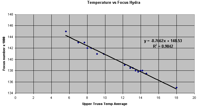
The plot below shows the change of the telescope focus with temperature, courtesy of Patricio Ugarte. The relationship can be used to provide a good guess at the focus for nights with poor seeing or partly cloudy conditions, and for an update of the focus during the night following temperature changes.
Last updated
There is a television camera in the telescope chimney which allows you to see the position of the comparison lamp mirrors, the corrector and everything else in the cage. It is good practice to turn it on before using Hydra to check and see if everything appears to be in the right place. In particular, the TV camera allows you to verify that the corrector has been deployed.
This camera is turned on from the TCS operator's console by going into the "command mode" and issuing the cryptic command:
local cfadc outlet1 move on
Be sure and turn it (and its associated light) off when you are finished! Use the command:
local cfadc outlet1 move off
The Hydra fibers are positioned within a 40' field approximately 380mm in diameter. Each fiber moves radially into the field from the periphery. A tiny prism is cemented to the tip of each fiber. The tip/prism assmebly is in turn cemented to a small magnetic button. Each button can be picked up and set down anywhere within a pie-shaped area emanating from its "Home" position just outside of the edge of the field.
Fibers are positioned with a "Gripper" which moves above the field on a high precision, computer controlled X-Y stage. The gripper is capable of a small amount of vertical (Z) motion. To move a fiber, the gripper jaws are opened. It is positioned over the fiber/button assembly, moves down, picks up the fiber and moves it to the target position with an rms precision of less than 10µ (.06"). The cycle is completely automatic and takes approximately 4 seconds per fiber.
There are 288 fibers, alternating between two sets each of which has 138 fibers and 6 spares. The "large" fibers are 300µ (2") in diameter. The "small" fibers are 200µ (1.3") in diameter. The small fibers were brittle and are not usable. Thus the instrument can position 138 2" fibers. A few are broken or have low throughput so that roughly 130 independent targets can be simultaneously observed.
The fibers are positioned on a flat plate. After they have been positioned, the plate is warped by applying a partial vacuum behind it, pulling it against some hard stops which hold it into a radius of 8.6M which conforms to the focal plane of the telescope. The telescope is "telecentric" meaning that the pupil is at the center of curvature of the field so that the light enters the fibers parallel to their optical axes.
The gripper stage carries a television camera so that you can see the gripper in action. Very occasionally the gripper drops a fiber. Should this happen to you, don't despair! It is usually not difficult to use the TV camera to find and recover a lost fiber. The procedure for doing so is described in the User Manual.
Last updated
Nick Suntzeff 20 March 2000. Updated by K. Olsen 3 May 2006. Revised by R. De Propis 27 Nov 2009.
La Serena personnel:
David James (Hydra scientist): x358
Rolando (Rolo) Cantarutti (computer software engineer): x373
Andres Montane (mechanical engineer): x309
Mountain support:
Observer Support x400 (Mauricio Rojas)
Observer Support x422 (Hernan Tirado)
Electronicos x417 (Humberto Orrego, Javier Rojas, David Rojas, Enrique Schmidt)
For setup questions prior to your run, contact Hydra scientist David James. Once on the mountain, contact Observer Support for help. ObsSup is on call from about 11am-midnight. Call them if you need to change a tilt, a filter, open the dome, etc. The telescope responsibility is handed off from ObsSup to the night assistant around sunset. If you need to do calibrations right at sunset (and you do!), you must communicate this to ObsSup in the afternoon, otherwise they may all be at dinner just at the time
LINK to hydrapro.tar file not found in the server
The best way to prepare for Hydra is to become familiar with the Hydra assignment program at home, and to come to Tololo a day in advance to see Hydra being used by the previous users.
Unlike most other instruments, Hydra requires that you come to the telescope with extremely accurate positions and a well planned program. We provide you with a simulator ("hydrasim") to do the assignments by hand or a Fortran program ("hydraassign") for a brain-dead way of doing the assignments.
See hydra software [18] for both of these programs.
While "hydraassign" works well, you may want to check the assignments with "hydrasim" and maybe tweak up the final assignment.
You need to have sky positions if you want to do sky subtraction. You can add sky positions by hand using the "hydrasim" program. In addition, I have a Fortran program that will make circles of sky positions at selected radii. Contact me (Nick) if you want the program. Knut has an IDL program that also does this. You can get it as part of a tar file of other programs from http://www.ctio.noao.edu/~olsen/IDL/hydrapro.tar [19].
The hardest part of the preparation is the measurement of astrometric positions. If your data come from Mosaic II [20], then you probably already have derived good positions for your targets. Just make sure that you've checked the accuracy of the astrometry in the header against the USNO-A2, USNO-B, or other catalog. The IRAF MSCRED package has tools to do this. If your images have no astrometry in them, then you'll have to make it from scratch. The IRAF IMCOORDS package will get you started. Frank Valdes also has a web page with nice instructions [21], which were written with Mosaic data in mind, but which are helpful for other kinds of data.
The format of the coordinate files that are input into the Hydra programs are Fortran fixed format. You must follow the formats exactly (in terms of column number) and *do not* go beyond the columns noted. Don't be creative here. Some common gotcha's during assignment:
You are now at the 4m observing room. Although the first two computers listed below are the ones that actually control the instrument, they should be hidden from you. We access them through virtual "VNC" windows (see "Starting VNC"), which we can run from any computer, although you are likely to run them from either ctiozm, ctioa7, or both. The benefit of doing things this way is that it allows us to see what you are doing from La Serena, and could even be used to allow collaborators to check up on you from their home institutions--please talk to us first if you would like to do this, however.
Generally one person will be the observer and operate the VNC windows. The other person will be doing assignments, bookkeeping, and totally useless web surfing (when the observer is not looking).
All the computers are auto-mounted and can see common disks. Thus, if the ctiozm or ctioa7 user has made an assignment file on the ctioa7 disk, this can be copied directly to a local disk on ctioa6. The only weirdness is that the ctioa6 disks cannot be seen by other users via automount. They can be accessed by scp, though. ctioa6 can see the disks of ctioa1, ctiozm, and ctioa7.
The computers should be set up for you. If not, here is what you do. Log into ctiozm, username "hydra". Then type "startx" to bring up the window manager.
==> After clicking on the Hydra GUI button located along the bottom panel on ctiozm, which brings up the VNC window, type "hydractio" in one of the black NTERM windows. There is no need to source it into background (with the "&"). The Hydra GUI will come up. It will ask you if you want to reload the previous coords. Unless you left the Hydra program with the fibers at a configuration position and want to continue to use this setup, answer this "NO." You will now be told to type "coldstart" in the white Hydra control window. Hydra is now ready for use.
TO LEAVE the program:
Under file, use QUIT.
==> Bring up the Arcon VNC window on ctiozm:
If it's not already running, right-click to bring up the menu and click on "(Re)Start Arcon". At this point it takes about 60sec for a dizzyingly large number of designer colored windows with mini-fonts to open. You will be asked a single question half-way through the process "Do you want to synchronize the parameters?" In the 6 years I have been using ARCON, I have always said "yes." I have no idea what happens if you say "no," but it probably involves pain and shouting. I think the question is there to see if you are awake.
I HATE the default fonts for the IRAF window. I edit the following line into IRAF section of the .openwin-menu:
| "IRAF" DEFAULT | exec | /local/combin/xgterm | ||
| -title | "IRAF" | \ | ||
| -geometry | 80x40 | \ | ||
| -bg | mistyrose\ | |||
| -fg | blac | \ | ||
| -sl | 600\ | |||
| -cr | darkred\ | |||
| +sb \ | ||||
| -fn | 10x20\ | |||
| -e | cl | |||
/local/combin/xgterm
==> You will probably want to run the Hydra simulator on ctiozm or ctioa7. If the latest version is not already installed, the user should immediately install the "hydrasim" software using the instructions at the hydra software page [24]
Load your coord and assignment files in some subdirectory in ctiozm or ctioa7 - I use "fields." Try entering one of your files into the simulator software to make sure everything is working.
THE CCD:
| slit 141 | ||||
| | | --------------------------------------- | | | ||
| | | | | |||
| red | | | | | blue | |
| | | | | |||
| | | | | |||
| | | --------------------------------------- | | | ||
| slit 0 |
ccdinfo:
cl> ccdinfo
| (gain = | 1) | Gain setting |
| (xsum = | 1) | pixels summed in spatial direction |
| (ysum = | 1) | lines summed in spectral direction |
| (xstart = | 1) | Start of ROI in X (in unbinned pixels) |
| (ystart = | 1) | Start of ROI in Y (in unbinned pixels) |
| (xsize = | 2048) | Size of ROI in X (in unbinned pixels) |
| (ysize = | 4096) | Size of ROI in Y (in unbinned pixels) |
| (extend = | "separate") | Method of extending ROI to include overscan |
| (noverscan = | 64) | Number of overscan pixels (binned) |
| (xskip1 = | 10) | X pixels to skip at start of overscan (binned) |
| (xskip2 = | 0) | X pixels to skip at end of overscan (binned) |
| (xtrim1 = | 0) | pixels to trim at start of data |
| (xtrim2 = | 0) | X pixels to trim at end of data |
| (ytrim1 = | 0) | Y pixels to trim at start of data |
| (ytrim2 = | 0) | Y pixels to trim at end of data |
| (preflash = | 0.) | Preflash time (seconds) |
| (pixsize = | 15.) | Pixel size in microns |
| (nxpixels = | 2048) | Detector size in X |
| (nypixels = | 4096) | Detector size in Y |
| (detname = | "SITe4096") | Detector identification |
| (mode = | "ql") |
|
*** Table of gain values*** SITe 2Kx4K + Arcon3.7 |
||||||||||
| Hydra Bench Spectrograph | ||||||||||
|
I n d e x |
D w e l l |
D e l a y |
----------------------------------------------- | |||||||
|
1/Gain (e-/ADU) |
Read Noise (e-) |
Full Well (e-) |
Spurious Charge (e-) |
Read Times | ||||||
|
2x1 (s) |
1x1 (s) |
2x2 (s) |
||||||||
| - | ---- | - | ------------------------------------------------ | |||||||
| 1: | 1 | 3000 | 3 | 2.36 | 5.2 | 60000 | 5.0 | 101 | 85 | 61 |
| 2: | 2 | 8400 | 3 | 0.84 | 3.0 | 15000? | 0.25 | 150 | 133 | 85 |
Spurious Charge is signal per pixel generated by clocking
the CCD. Read Noise is quoted for overscan pixels. In the image:
Noise floor = sqrt{ Read_Noise^2 + xbin * ybin *
(Spurious_Charge + Dark_Current * Exposure_Time) }
Dark current = 0.7 e-/hr (per unbinned pixel) in Jun, 2001,
at CCD_TEMP= 150K (pumped N2, heater off)
For gain 2, bin 2x2, total noise in 1800 sec dark = 3.5 e-
Read times are quoted for binning (spatial x spectral).
When binning 2x2 the ADC saturates before full well is reached.
NB: A peculiarity of this CCD is that full well is highly
variable from pixel to pixel causing vertical trails to
to appear at high signal levels. The full well figures are
very preliminary estimates for the worst pixels.
*** Select gain setting from the first column
*** The current gain setting is 1
During the night, at every slew position and every configuration: (these are typical numbers) echelle: etalon, 180s; quartz, 120s rc mode: penray 10s, quartz 10s for KPGL3
Note that "penray" is actually a rack of a number of lamps, including neon, helium, argon, and xenon. It is supposed to emulate a more traditional (but much dimmer) he-ne-ar lamp. The line ratios are very different from those in the old lamps. The henear lamp is available but is dim and not very dense in lines.
During the day: (do all these with the fibers at the large circle position:
select "File->Run Script->largecircle (or configlargecircle)->Open" from the
menu bar in the Hydra GUI, or type "execfile largecircle" in the command window)
25 biases
echelle:
3 daytime skies @ 45s + etalon (with dome closed!)
3 th-ar, 600s
3 penray,henear, 300s
darks (I ususally leave darks running at the end of the night when I
go to bed)
rc mode:
10 dome flats (make sure that you tell ObsSup that you want the color
balance filters removed to do these. We have some blue color
balance filters on the flat-field lights on the ring of the telescope
for direct CCD work. These must be removed)
3 penray, 1s
3 twilight skies (right after sunset)
During the run once:
milky flats
The ObsSup will be more than happy at the chance to install the milky flat diffusing screen in the spectrograph. To do the milky flats, you have to bring in the fibers to the large cicle. Do this by selecting the "largecircle" script from the File->Run Scripts menu. Do the milk flats.
You may want to take some short exposures of the milks to get data for the mask image. The division of the short milk and the long milk is a good way of revealing the traps and bad pixels.
I STRONGLY suggest you worry about the dark frames. You should verify that the dark count is low. The CCD should have only a few e-/hr/pixel behind a dark slide. The spectrograph is wide open, and although we try as hard as possible to keep stray light out, sometimes doors aren't closed and light gets in. The dark count should be no more than 10e-/pix/hour. The Mosaic CCD chip should have less than 3e- read noise, so any dark more than ~10e-/pixel in your exposure is going to reduce the S/N of a faint object.
In the Arcon parameter file "instrpars", set the "lampsys" parameter to "new" and select the comparison lamp you want to use in "complamp", using "pen" for the HeNeArXe penray. When you take a comparison lamp exposure (through "comp" or "observe"), the Arcon will automatically move the system into place and turn on the lamps. You can watch all this happening from the "Lamps" menu in the Hydra GUI. Note that Arcon will turn off the lamp but leave all the mirrors, etc. in place after the exposure is finished. If you go to a field and can't see any stars through the gripper camera, you've likely forgotten to park the comparison lamp system. Do this from the Hydra GUI by clicking the "Park" button.
MAKE SURE THAT THE GRIPPER IS OUT. IF THE SOME OF THE SPECTRA ARE MISSING, IT IS PROBABLY THE GRIPPER IN THE WAY.
It is not too difficult to focus the telescope using the FOPS. You can ask the night assistant to focus for you and he (she) will use the following procedure. Remember that the FOPS are fiber bundles of 7 1 arcsec fibers. Choose a single FOPS with a star on it near the field center. The idea is to get most of the light into the central fiber by changing the focus.
The object will move during focus and the FOPS will lose centration. I found to focus, you must do the following:
Typical values:
12.8 degrees 156200
If you are using echelle more or observing longward of 6000A and need high S/N spectra, you probably need a telluric standard. It is best to do it through a few fibers. You can do it one fiber and exposure at a time. Alternatively you can bring in a number of fibers sequentially. Put the fibers at the large circle or park position. Bring one fiber into the center. Start a long exposure on the CCD (3600s). Expose for say 100s and then "pause". Then:
unwarp
gripin
park 000
move 001 0 0 <== some other fiber here.
warp
gripout
and expose for 100s starting with "resume" on CCD window. Etc. (Check to see if light is leaking in from gripper light.) You can do this on about 4-6 fibers with the telescope in open loop tracking.
Alternatively, you can put a FOPS down on one guide star (and have the object in the center). After moving the a new fiber to the center and warping the plate, recenter the guide star on the FOPS. You can turn on the FOPS guider to guide, but I recommend just guiding by hand on these short exposures.
You can get the *.hydra fibers of the tertiary spectrophotometric standards of Baldwin and Stone (1984, MNRAS, 206, 241; 1983, MNRAS, 204, 347) as calibrated at CTIO by Hamuy et al. (1992, PASP, 104, 533; 1994, PASP, 106, 566). These are 11-14th mag stars. I also have *.hydra fields for the secondary spectrophotometric standards (also called Hayes standards) as give in the Hamuy reference. These have fluxes every 16A. The stars are 4-6th mag.
The coords are taken from USNO-A2.0 and have the standard in the center with FOPS stars and skies scattered around in the field. See the directory:
/uw52/nick/hydra/text/specphot/*.coo
A selected list of bright, hot stars culled from the Yale Bright Star Catalog can be found in:
/uw52/nick/hydra/text/bstar.dat
Basic CCD reductions. The idea here is to process the ALL THE SPECTRAL DATA, including the object, pflat, dflat, and sflat data, to [OTZF] before extracting.
Find the biassec and trimsize. You must trim out as much of the image as you can to make the flat fielding as easy as possible. Process the data through [OTZ].
ccdr:
| (pixeltype = | "real real") | Output and calculation pixel datatypes |
| (verbose = | yes) | Print log information to the standard output? |
| (logfile = | "logfile") | Text log file |
| (plotfile = | "") | Log metacode plot file |
| (backup = | "") | Backup directory or prefix |
| (instrument = | "ccddb$ctio/csccd.dat") | CCD instrument file |
| (ssfile = | "home$/subsets") | Subset translation file |
| (graphics = | "stdgraph") | Interactive graphics output device |
| (cursor = | "") | Graphics cursor input |
| (version = | "2: October 1987") | |
| (mode = | "ql") | |
| ($nargs = | 0) |
ccdpr: (last half of n2 and n3)
| images = | "sflat*" | List of CCD images to correct |
| (ccdtype = | "") | CCD image type to correct |
| (max_cache = | 0) | Maximum image caching memory (in Mbytes) |
| (noproc = | no) | List processing steps only?\n |
| (fixpix = | no) | Fix bad CCD lines and columns? |
| (overscan = | yes) | Apply overscan strip correction? |
| (trim = | yes) | Trim the image? |
| (zerocor = | yes) | Apply zero level correction? |
| (darkcor = | no) | Apply dark count correction? |
| (flatcor = | yes) | Apply flat field correction? |
| (illumcor = | no) | Apply illumination correction? |
| (fringecor = | no) | Apply fringe correction? |
| (readcor = | no) | Convert zero level image to readout correction? |
| (scancor = | no) | Convert flat field image to scan correction?\n |
| (readaxis = | "line") | Read out axis (column|line) |
| (fixfile = | "") | File describing the bad lines and columns |
| (biassec = | "[1:55,1:1004]") | Overscan strip image section |
| (trimsec = | "[75:3120,1:1004]") | Trim data section |
| (zero = | "home$n3/biasn3") | Zero level calibration image |
| (dark = | "") | Dark count calibration image |
| (flat = | "home$n3/flatn3") | Flat field images |
| (illum = | "") | Illumination correction images |
| (fringe = | "") | Fringe correction images |
| (minreplace = | 1.) | Minimum flat field value |
| (scantype = | "shortscan") | Scan type (shortscan|longscan) |
| (nscan = | 1) | Number of short scan lines\n |
| (interactive = | no) | Fit overscan interactively? |
| (function = | "legendre") | Fitting function |
| (order = | 10) | Number of polynomial terms or spline pieces |
| (sample = | "*") | Sample points to fit |
| (naverage = | 1) | Number of sample points to combine |
| (niterate = | 3) | Number of rejection iterations |
| (low_reject = | 2.5) | Low sigma rejection factor |
| (high_reject = | 2.5) | High sigma rejection factor |
| (grow = | 0.) | Rejection growing radius |
| (mode = | "ql") |
To process milk flats, first process through [OTZ]. The idea here is to bring the milk flat to 1.0 everywhere with the pixel to pixel variation left in. If a few wiggles are left in the image, that's okay. You will be dividing by the dflats later anyway. To bring the milky flat to 1.0, you need to remove the faint ripples of the fiber images. These run along the x-axis. The trick to remove these is to create a median filtered image using a long skinny boxcar and divide this into the data.
Do something like:
imdel temp*
# combine the milky flats into a single image
comb @in1 temp1
# remove the spectral shape in the x-direction
blkavg temp1 temp2 1 2000
fit1d temp2 temp3 fit ax=1 low=2 high=2 or=20 niter=10
blkrep temp3 temp4 1 1004
imar temp4 / 2000 temp4
imar temp1 / temp4 temp5
# remove the spectral shape in the y-direction
blkavg temp5 temp6 4000 1
fit1d temp6 temp7 fit ax=2 low=2 high=2 or=3 niter=5
blkrep temp7 temp8 3021 1
imar temp8 / 2000 temp8
imar temp5 / temp8 temp9
# filter the data with a long skinny boxcar
fmed temp9 temp10 xwin=51 ywin=1
imar temp9 / temp10 flat
(you may want to process with fmed in y direction also)
Now process through [OTZF]. MAKE SURE THAT YOU PROCESS THE PFLATS, SFLATS, DFLATS, AND COMPARISONS. YOU MUST CHANGE THE "IMAGETYP" TO "OBJECT" FOR THE PFLATS AND THE SFLATS TO GET THEM TO FLATTEN.
We have four types of lamps:
Helium-Neon-Argon (a single lamp with all 3 gases)
"Penray" which is actually 4 lamps of helium, argon, neon, and xenon.
The individual lamps in the penray "lamp" can be turned on or off on the hydra instrument (but not from the Hydra GUI). All lamps should be on. We have been having problems with the neon lamp burning out or being weak.
Thorium-Argon
etalon
The wavelengths are kept in the IRAF directory linelists$. Some additional notes if you want to go to the original sources:
For the Xenon lines, use the list in Striganov & Sventitski, "Tables of Spectral Lines of Neutral and Ionized Atoms", 1968, (IFI/Plenum: New York). This is a good source for all wavelenghts in the visible region and is accurate enought for all the RC setups. It is a nice table because it gives intensities also.
The best source for argon lines is: Norlen, 1973, Phys. Scrip. 8, 249.
The thorium lamp has rather weak thorium with respect to argon, and the lamp seems to have a quite different ionization than typical atlases for th-ar, such as the ESO atlas. Very accurate wavelengths are given in: Palmer, B.A., and Engleman, R. Jr. Los Alamos Sci Lab Pubs, LA-9615. In the blu, the ThAr lamp is basically all argon, with only the very brightest Th lines appearing weakly in the spectra.
In the blue, the He lines dominate in the penray lamps.
As far as I can tell, there is no neon in the he-ne-ar lamp.
See Knut's reduction notes [25].
We have DDS3 and exabyte. We also have DLT 7000, but you will not be generating that much data to need a DLT. Most people write data to tape using the IRAF "wfits" command. This is not a particularly efficient way to write data, but it is tried and true. I would NOT recommend writing a large tar file. A tape error in the middle of a tar read can ruin your whole day because it is hard to force the tar past the bad data point (if this happens, turn off the parity checking in the tar command). If you do write tar, I recommend breaking the data up into tar files = say one per night of no more than 1-2 Gbyte.
Write two tapes just in case. Give one to your collaborator or sister or whoever, just in case. Data can be (painfully) recovered from the SAVE THE BITS backup tapes, so if you can't even read your sister's tape, you can ask us to recover it from the backups.
DON'T PANIC
These are common problems with simple solutions.
You get an error while configuring where an annoying little grey box pops up and says: "Error:configure: OrderMoves Error: phys move. MoveButt couldn't pick up button xxx" where xxx is some fiber name.
What has happened is that the gripper has gone to the position of xxx and could not pick up the button. Much of the time this is because the button is slightly off from where it should be, possibly because it was placed down on a small piece of dust. Sometimes too much stress builds up in the hypodermic needle which houses the fiber and the fiber simply slides out of the gripper.
However a fiber might get lost, to recover use the gripper TV to place the gripper on top of the fiber. Then, in the command window, type "thisis". This tells the software that the gripper is on top of whichever fiber is currently lost. Note the use of small letters in this command. (The related command "ThisIs xxx" tells the software explicitly that fiber xxx is under the gripper.)
If the fiber is not visible in the gripper TV, you can use the GUI to cruise near where it should be and see if you can find it. If you find it, tell the gripper where it is using the "thisis" command. Don't go very far cruising or you may find another button and get Hydra really mixed up by identifying it incorrectly.
If you can't find the lost fiber near the nominal position, return the gripper to the "parked" position of the lost fiber. There is a good chance that the fiber will be there and was never picked up in the first place.
If the fiber is not in the parked position, you will see the hypodermic tubing enclosing the fiber crossing the field going to wherever the button actually is. Use the gripper motion controls to follow the tube out into the field until you find the button, put the gripper on top of it and then use the "ThisIs" command to tell Hydra where it is.
If the button appears tilted there is sometimes a tiny piece of ferrous material stuck to the bottom. There may be damage to the button. In either case if this happens, call Observer Support and have them inspect and retire the fiber manually.
Once the fiber is returned to the park position, you can use it again. If it keeps on getting lost, you should lock it and not use it for the rest of the run.
If the fiber is really totally lost, or this procedure doesn't work, you will have to have Observer Support come and retire the fiber manually.
You were able to configure the program with hydrasim, but you get an error about a transformation problem when doing the real configuration. This error happens just after you start the configuration.
What is happening here is that the hydra program is doing one extra step beyond the hydrasim program. It is taking the coords and assignments, and appplying a transformation to the appropriate zenith distance for the observations. For some reason, the transformation is producing a collision.
Possible causes:
Everyone has their own programs to generate the Hydra assignment files with the right formats. I use some IDL programs that I have written:
IDL>readcol,'file.dat',name,ra,dec,f='A,A,A'
IDL>hydcoo,name,ra,dec,replicate('O',n_elements(ra)),epoch=2000.0,fname='FIELD 1',fileout='field1.coo'
IDL>tycho2hyd,'field1.tycho',fileout='field1fops.coo',mlo=10,mhi=12,skyrad=[5,10,15,20],nsky=20
I then merge the HYDCOO and TYCHO2HYD outputs into a single coordinate file for feeding into hydraassign.
Download tar file of IDL programs
How useful are all those flats? Here's what I've been doing:
Comparisons: I like to have a comparison adjacent to every object exposure, so that the observing sequence goes like this: comparison-object-object-comparison-object...
Preliminary steps:
Extractions with dohydra:
dohydra obj029c apref=pflat028 flat=dflat016 throughput=sflat020 arcs1=comp030 readnoise=3. gain=0.84 datamax=65000. fibers=107 width=12. minsep=6. maxsep=14.1 crval=4950. cdelt=-1.2 objbeam=0,1 skybeam=0 scatter- fitflat+ clean- dispc+ savearc- skysub+ skyedit+ savesky- splot+
dohydra will take you through aperture identification (check it carefully!), aperture tracing, fitting of the flat field spectrum, arc lamp identification and dispersion correction, and sky subtraction. Sky subtraction can be tricky; if your spectrum is heavily contaminated by night sky emission lines, you may have to be more creative than dohydra allows. As a result, the above recipe works fairly well in the blue, but may fail in the red.
KAO 17 Aug 2002
This is a brief introduction describing how we use VNC (Virtual Network Computing) [29] to display the various windows which control use of the Hydra CTIO spectrograph. The advantage of using VNC is that support staff (both on the mountain and downtown) can monitor the use of the instrument, actually SEEING in real time any errors that appear. It also lets the observer control both the Arcon and the Hydra GUI from the same keyboard.
First, log into ctiozm with the username hydra (ask the night assistant or Observer Support for the password. Once logged in, click on the README button at the bottom of the screen. This will open a file showing you how to get started.
If Hydra has been up and running, you should only have to click on the Hydra GUI and Arcon window buttons, as the README file says. (These buttons run scripts which reside in /ua80/hydra/bin/: start_a1, view_a1, start_ja, and view_ja, which are named to refer to the computers ctioa1 and ctioa6 which operate Arcon and the Hydra software, respectively).
In short order, two windows should appear. In the tall rectangular window (ctioa1), right click in the desktop to bring up the menu and click on "(Re) Start ARCON Session". In the wide rectangular window (ctioa6), right click in the desktop, move the mouse onto the "Hydra" menu, and click on "Start Hydra Gui". The following images show what should be the result of the instructions above. Click on either for a larger view.
If pressing the buttons produces no result, or the VNC clients start up but the menus appear inaccessible, you will probably have to kill the servers and restart them manually, as follows.
On ctiozm, open an xgterm or xterm window. All of the following commands below (where it says "type...") should be typed into this window.
1. rsh ctioa1 "source .login; vncserver -kill :9"
2. rsh ctioa1 "source .login; vncserver :9 -depth 8 -cc 3 -alwaysshared -geometry 670x864"
This should start the vncserver on ctioa1 and output the following text:
New 'X' desktop is ctioa1:9
Starting applications specified in /arc/hydra/.vnc/xstartup
Log file is /arc/hydra/.vnc/ctioa1:9.log
If line 2 generates an error message about a file in /tmp, remove the file (rsh ctioa1 "rm /tmp/file_name") and try line 2 again.
Clicking the "Open Arcon VNC viewer" button should now bring up the Arcon VNC viewer. If you would rather start the viewer manually ,too, then type
vncviewer ctioa1:9 -passwd /ua71/hydra/.vnc/passwd &
The VNC viewer window should come up, and something like the following output should show up in the xgterm where you typed vncviewer.
VNC server supports protocol version 3.3 (viewer 3.3)
VNC authentication succeeded
Desktop name "hydra's X desktop (ctioa1:9)"
Connected to VNC server, using protocol version 3.3
VNC server default format:
8 bits per pixel.
Colour map (not true colour).
Using default colormap which is TrueColor. Pixel format:
16 bits per pixel.
Least significant byte first in each pixel.
True colour: max red 31 green 63 blue 31, shift red 11 green 5 blue 0
Using shared memory PutImage
1. rsh ctioa6 "vncserver -kill :9"
2. rsh ctioa6 "source .login; vncserver :9 -cc 3 -alwaysshared -geometry 810x700;"
This should start the vncserver on ctioa6 and output the following text:
New 'X' desktop is ctioa6:9
Starting applications specified in /ua71/hydra/.vnc/xstartup
Log file is /ua71/hydra/.vnc/ctioa6:9.log
Again, if starting the server produces an error message, remove the appropriate file in /tmp and repeat step 2. Clicking the "Open Hydra GUI viewer" button should now bring up the VNC viewer. If you would rather start the viewer manually, type
vncviewer ctioa6:9 -passwd /ua71/hydra/.vnc/passwd &
The VNC viewer window should come up, and something like the following output should show up in the xgterm where you typed vncviewer.
VNC server supports protocol version 3.3 (viewer 3.3)
VNC authentication succeeded
Desktop name "hydra's X desktop (ctioa6:9)"
Connected to VNC server, using protocol version 3.3
VNC server default format:
8 bits per pixel.
Colour map (not true colour).
Using default colormap which is TrueColor. Pixel format:
16 bits per pixel.
Least significant byte first in each pixel.
True colour: max red 31 green 63 blue 31, shift red 11 green 5 blue 0
Using shared memory PutImage
Sometimes VNC doesn't gracefully let go of the X display it is using (sometimes for a few minutes, sometimes longer). If, for example, one of the VNC servers crashes (which I've never seen happen), and the user immediately tries to restart it, one may get an error saying that VNC is running on :9, even though it isn't. Such an error might look like
hydra@ctiozm [30]% start_a1
A VNC server is already running as :9
[1] 3328
vncviewer: ConnectToTcpAddr: connect: Connection refused
Unable to connect to VNC server
[1] Exit 1 vncviewer ctioa1:9 -passwd /ua71/hydra/.vnc/passwd
To get around this problem, first try waiting about 2-3 minutes before starting the server again. This should be enough time to allow the socket to be released. If this fails repeatedly, try going through the manual startup and substitute another number, for example 8, whereever you see 9 in the above manual example. This will start up the VNC sessions on X display :8, but otherwise should be the same.
You can bypass VNC completely and start up the windows directly. To do this...
This should bring up the normal Arcon windows directly on the ctioa1 display, and the Hydra GUI on ctioa6.
To connect from other machines, you must (of course) have the VNC viewer application installed. This should be installed on most workstations, and can be downloaded for PCs and Macs from the VNC Homepage [29].
To view a Hydra session, simply use the VNC viewer application to connect to ctioa1:9 (for the Arcon windows) or ctioa6:9 (for the Hydra GUI). You must know the password to enter. NOTE!! You should ALWAYS enter as VIEWONLY unless you are trying to remotely help the observer. If you do not know how to do this, DON'T CONNECT!
Please send comments and questions to: Roberto De Propris: rdeproprisATctio.noao.edu Last updated: 2 May 2006 by Knut Olsen
A CTIO Hydra simulator is available for observers to learn how to use Hydra. There are versions for both Linux and Solaris. The Linux version is known to run on Red Hat 6.1+ and S.U.S.E. 6.2+. It probably runs under most new versions of Linux but we have not tested it on any other distribution. We would appreciate observers who try it on other Linuxes to let us know whether it does or does not work.
If you want to use it, point your browser here [31]. It is also available from the CTIO ftp mirror at NOAO Tucson [32] (updated nightly).
Any comments or suggestions are always welcome! Send them to rcantaruttiATnoao.edu
As far as we know, the simulator works fine. Please let us know if you have any problems. If you don't want to bother downloading the simulator, you can get some idea of what you are dealing with by looking at the most recent CTIO Hydra GUI. [33]
IMPORTANT: If you are using the simulator to prepare for an observing run, be sure to install the latest version since the Hydra code is continuously being upgraded. A new simulator is always generated when the working software is updated. Any version can be used for practice, but if one is generating assignment files for real observing, the simulator must be the same version as the Hydra program itself or the assignments may not work.
When using the simulator for generating assignment files please be sure that the time set in the simulator is the same as the time at which you anticipate the observations will actually be made. If the time is set incorrectly, atmospheric refraction corrections can produce assignment files which will cause unexpected collisions or ask Hydra to go to unattainable configurations.
Hydra-CTIO GUI runs on ctioa6 and connects to the Hydra instrument through an RS-422 serial line. The ctioa6 machine is also connected to the local ethernet network allowing Hydra GUI to request status and send commands to the TCS [34] through the GWC router.
The FOPS Guider machine is also connected to the local ethernet network allowing Hydra-CTIO to send direct commands to enable/disable guiding. The FOPS Guider machine send the guiding command thorugh an RS-232 serial line to the TCS program running on ctiox0.
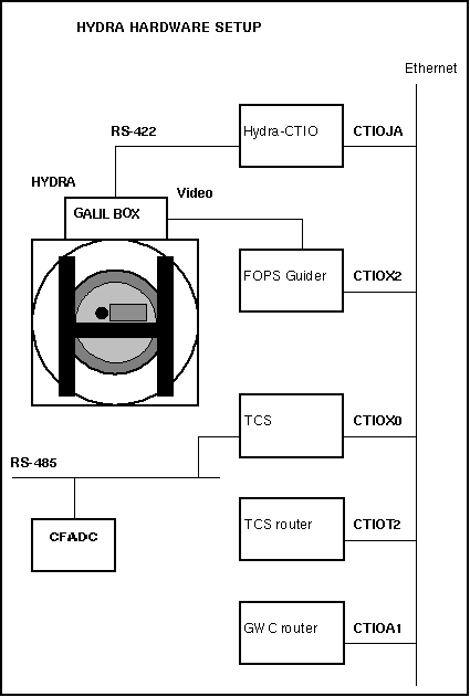
The TCS program running on ctiox0 doesn't have native support for the GWC libraries so an auxiliary program running on ctiot2 provides that support. The program running on ctiot2 is called tcsrouter [35] and basically routes messages from other applications, coming through the router, to the TCS.
This function is called on system reset. It's a special label (Galil Firmware) to create an autostart program on power-up. Everything starts from here. One of it's main functions is to flag that nothing is initialized. Various functions read the variable "Reboot" and terminate if it is non zero. Other functions are to lock the brakes and turn the drives off.
File: main.g
Args: (none)
Results: (none)
Messages sent to the Mid-level code: (none)
Embedded functions called from this one:
JS #Brakes
JS #DbCreat
JS #Temp
This function locks/unlocks the brakes on the x/y gantry.
File: xyops.g
Args:
BraARG1 -- Lock/unlock flag
0 = lock Brakes
<> 0 = un-lock Brakes
Results:
BraRSLT1
0 = No Error.
>0 = Gallil error code resulting from "OB" command.
Messages sent to the Mid-level code:
(normal)
MG "boxBrakes set state starting"
MG "boxBrakes set mode locked"
MG "boxBrakes set mode unlocked"
MG "boxBrakes done"
(errors)
MG "boxBrakes set result error"
MG "boxBrakes set error NoBrakes"
This function closes the gripper. It then tests for button presence. It takes no arguments and set two different result variables before it exits. Result variable CloRSLT1 is set to the result of closing the gripper. Result variable CloRSLT2 is set to zero if the gripper is empty after closing the jaw. If after closing the jaw a button is present CloRSLT2 is set to one.
File: gripops.g
Args: (none )
Results:
CloRSLT1 Result of closing gripper.
0 = No error, i.e. closed
2-99 = Error. Value from galil "SC" command.
CloRSLT2 Button presence after gripper close.
0 = Gripper empty
1 = Button in gripper
Messages sent to the Mid-level code:
(normal)
MG "boxClose set state starting"
MG "boxClose set result ok"
MG "boxClose set mode closed"
MG "boxClose done"
(errors)
MG "boxClose set result error"
MG "boxClose set error NoClose"
Embedded functions called from this one: (none)
This function traps command errors and causes them to retrun an error code to whatever function happened to be running at the time. Basically this is a "I forgot to test for it" trap.
File: main.g
Args: (none)
Results: (none)
Messages sent to the Mid-level code: (none)
Embedded functions called from this one: (none)
This function starts up the system. First, the system is put in a safe state. Next the satus monitor is started up. Finally, the initialization functions (init and home) for each axis are called with safety checks along the way. The initialization will abort if there is an unexpected error.
File: coldstart.g
Args:
ColARG1 = Level of safety override
0 = No safety overrides.
1 = Initialize with a button present.
Results: (none)
Messages sent to the Mid-level code:
(normal)
MG "boxCold set state starting"
MG "boxCold set result ok"
MG "boxCold done"
(errors)
MG "boxCold set result error"
MG "boxCold set error ButtonOnInit"
MG "boxCold set error ButtonNotID"
MG "boxCold set error GripInit"
MG "boxCold set error NoStatMon"
MG "boxCold set error NoGripInit"
MG "boxCold set error NoZInit"
MG "boxCold set error NoXYInit"
MG "boxCold set error UnknownErrInit"
Embedded functions called from this one:
JS #Ginit -- initializes the gripper axis
JS #Ghome -- homes the gripper axis
JS #IfButt -- see if a button is present
JS #Zinit -- initializes z axis
JS #Zhome -- homes the z axis
JS #XYinit -- initializes xy gantry system
JS #XYhome -- home the xy gantry system
This function drops up a button on the plate using the user supplied argument to decide how much to descend on the z axis. It determines the Z distance based on current radius from the center of the plate. Set argument variable DroARG1 to zero to compute the drop height based on x/y position. Set GraARG1 to 1 to assume drop on plate. Set GraARG1 to 2 to assume drop on park circle.
File: gripops.g
Args:
DroARG1 = Plate distance. See comment block above.
0 = Compute drop height from x/y position
1 = Assume drop on plate.
2 = Assume drop on park circle.
Results:
DroRSLT1 = Result of attempt to drop button.
0 = No Error.
1 = button still in gripper.
2 = Motion error
3 = Bad Argument
DroRSLT2 = Z status after dropping.
0 = No Error.
>1 = Galil "SC" result for last z move
DroRSLT3 = griper status after dropping.
0 = No Error.
>1 = Galil "SC" result for last gripper move
Messages sent to the Mid-level code:
(normal)
MG "boxDrop set state starting"
MG "boxDrop set result ok"
MG "boxDrop done"
(error)
MG "boxDrop set result error"
MG "boxDrop set error GripInop"
MG "boxDrop set error NotDropped"
MG "boxDrop set error zInop"
MG "boxDrop set error BadArg"
Embedded functions called from this one:
#Open -- opens the gripper
#Close -- closes the gripper
This function computes the encoder position from the distance between two reference marks. Note that this algorithm is specific to the Heidenhain Encoders. Variable names follow those in the documentation from the manufacturer.
The basic premise of this scheme is that index marks can be positioned in such a way that one only need traverse two of them and knowing the direction of travel, the absolute position of the first mark encountered can be determined.
The xhome, whome, and yhome routines all call this function as they all use the same type of encoder. This is a generic routine for any encoder of this type.
Note that this function is used internally and sends no messages back to the mid level code.
One should read the encoder documentation and the source for a complete understanding of how these routines work.
Args:
encARG1 = encoder position of 1st index mark encountered
encARG2 = encoder position of 2nd index mark encountered
encARGz = direction of travel
Results:
encRSLT1 = result of encoder formula.
This function turns the electronic box cooling fan on/off. Set the argument variable FanARG1 to zero if you want to turn the fan off, and set it to one if you want to turn the fan on. The function use output 16 of the Galil Box to command the fan.
File: periphio.g
Args:
FanARG1
0 = Fan Goes off
1 = Fan Goes on
Results: (none, just writes an i/o bit)
Messages sent to the Mid-level code:
MG "boxFan set state starting"
MG "boxFan set mode 0"
MG "boxFan set mode 1"
MG "boxFan set result ok"
MG "boxFan done"
Embedded functions called from this one: (none)
This function handles the hardware "error" interrupt. This interrupt is assigned to input 5.
File: errors.g
Args: (none)
Results: (none)
Messages sent to the Mid-level code: (none)
Embedded functions called from this one: (none)
This function homes the Gripper axis. First it checks to see if it's already into the home switch. If so, it backs out of it. Then it jogs slowly into the switch.
File: gripops.g
Args: (none)
Results:
GhoRSLT1 = 0 % Result code.
0 = No error
Messages sent to the Mid-level code:
(normal)
MG "boxGhome set state starting"
MG "boxGhome set result ok"
MG "boxGhome done"
(error)
MG "boxGhome set result error"
MG "boxGhome set error NoHome"
Embedded functions called from this one: (none)
This function initializes the gripper axis. Every time this function is called it loads the GripPos array. Then configures the encoders and motor type for G and enable the motor.
File: gripops.g
Args: (none)
Results:
GinRSLT1 = Result of homing gripper.
0 = No error
Messages sent to the Mid-level code:
MG "boxGinit set state starting"
MG "boxGinit set result ok"
MG "boxGinit done"
Embedded functions called from this one: (none)
This function picks up a button from the plate using the user supplied argument to decide how much to descend on the z axis. It determines the Z distance based on current radius from the center of the plate. Set argument variable GraARG1 to zero to compute the distance based on x/y position. Set GraARG1 to 1 to assume gripper is over the plate. Set GraARG1 to 2 to assume gripper is over the park/stow area.
File: gripops.g
Args:
GraARG1 = What height to use
0 = Compute z distance based on x/y position
1 = Assume gripper is over the plate
2 = Assume gripper is over the park/stow area.
Results:
GraRSLT1 = Result code.
0 = No Error.
1 = Gripper Inoperative.
2 = No button found.
Messages sent to the Mid-level code:
(normal)
MG "boxGrab set state starting"
MG "boxGrab set result ok"
MG "boxGrab done"
(errors)
MG "boxGrab set result error"
MG "boxGrab set error GripInop"
MG "boxGrab set error NotFound"
MG "boxGrab set error BadArg"
Embedded functions called from this one:
#Open -- opens the gripper #Close -- closes the gripper
This function Determines if a button is in the gripper. It first insures that the gripper is configured such that the test is valid. Under the present design, this means closing the jaws, and returning the result of the close operation. Later, it might be possible to detect a button no matter what the state of the gripper, and this function would be modified accordingly.
File: gripops.g
Args: (none)
Results:
IfBRSLT1 = Result of test for button.
0 = No Button.
1 = Button in gripper.
>1 = Gripper Error ( See "Close" )
Messages sent to the Mid-Level code:
(normal)
MG "boxIfButt set state starting"
MG "boxIfButt set mode nobutton"
MG "boxIfButt set mode button"
MG "boxIfButt set result ok"
MG "boxIfButt done"
(errors)
MG "boxIfButt set result error"
MG "boxIfButt set error NoClose"
Embedded functions called by this one:
#Close -- closes the gripper
This function is reserved by the box as the input intterupt handler. If any of the input interrupts have been enbled by the "II" command, this routine will called when the associated input bit goes low. From there, this routine will poll to see what needs service. "Reboot" and terminate if it is non zero.
File: main.g
Args: (none)
Results: (none)
Messages sent to the Mid-level code: (none)
Embedded functions called by this one: (none)
This function allows a user to reenable interrupts after an error.
File: errors.g
Args: (none)
Results: (none)
Messages sent to the Mid-level code: (none)
Embedded functions called by this one: (none)
This function read back the vacuum sense switch on the plate. It takes no arguments. The current on/off state of the sense switch is returned in result variable IsWRSLT1. The function reads analog input 9 to check the switch out.
File: periphio.g
Args: (none)
Results:
IsWRSLT1 = sense sqitch status.
0 Plate is flat.
1 Plate is warped.
Messages sent to the Mid-level code:
MG "boxIsWarpd set state starting"
MG "boxIsWarpd set mode", IsWRSLT1 {F2.0}
MG "boxIsWarpd set result ok"
MG "boxIsWarpd done"
Embedded functions called from this one: (none)
This function turn the gripper LED on to the specified level (Or else off....). Set argument variable LedARG1 to the desire level of intensity. A value of zero will turn the gripper LED off. The function uses the lowest 3 bits of I/O port 0 on the Galil Box to select the desired level (mask used with "OP" is 65532 or "1111 1111 1111 1000").
File: periphio.g
Args:
LedARG1 = intensity level.
0 = Led off
1 = On, low
2 = On, medium
3 = On, high.
Results: (none, just sets IO bits)
Messages sent to the Mid-level code:
MG "boxLed set state starting"
MG "boxLed set result ok"
MG "boxLed done"
Embedded functions called by this one: (none)
Caution: This page is meant to be an abstract of calling conventions and function behavior and does not document the details of the code.
The #Move function moves a fiber from one location to another as specified in the arguments. This is the fundemental function of the system, and all other functions are secondary to this one.
Pre-move safety checks include making sure of no collisions, valid destination, and no button presence in the gripper. All this checkings must be made by the mid/high-level code before moving a fiber. If you are using this function directly then be very careful because no safety checks are made by this function.
Next, the gripper travels to the button (see the functions in "xyops.g"), and attempts to grab it. (documented with the file "gripops.g") If successful, the gripper relax and the button is carried to the new location, and an attempt made to drop it. If the drop fails, the button can be parked directly from the gripper.
File: buttmove.g
Args:
MovARG1 = x current location
MovARG2 = y current location
MovARG3 = x destination location
MovARG4 = y destination location
Results:
MovRSLT1 = Result code. Note that 0-4 are same as button status.
0 = No Error.
1 = Locked.
2 = Not found
3 = Dropped
4 = Positioner not operational
5 = Last move not yet broadcast.
6 = Could not drop
7 = X,Y Motion Failure
8 = Button present on entry
9 = Database has not been initialized since reboot
Messages sent to the Mid-level code:
(normal)
MG "boxMove set state starting"
MG "boxMove set state seek"
MG "boxMove set state grab"
MG "boxMove set state carry"
MG "boxMove set state drop"
MG "boxMove set result ok"
MG "boxMove done"
(errors)
MG "boxMove set error FibLocked"
MG "boxMove set error NotFound"
MG "boxMove set error LostInTransit"
MG "boxMove set error PosNotOp"
MG "boxMove set error LastNotBroadcast"
MG "boxMove set error NotDropped"
MG "boxMove set error NoXYmove"
MG "boxMove set error GripNotEmpty"
MG "boxMove set error DbaseUndef"
Embedded functions called from this one:
JS #IfButt -- see if a button is present.
JS #xygo -- the xy move function
JS #Grab -- pick up the button.
JS #xygo -- the xy move function
JS # IfButt -- see if a button is present.
JS #Drop -- drop the button.
This function opens the gripper. The user supplied argument is used to determine the final position. If OpeARG1 is 0 then the final position will be "closed". If set to 1 the final position will be "relaxed". If set to 2 final position will be "normal open" position. If set to 3 the final position will be "open wide" position. This are the same values used in the array GripPos.
File: gripops.g
Args:
OpeARG1 = Position to open gripper to.
0 = Closed position
1 = Relaxed position
2 = Normal open position
3 = Open wide position
Note that the values used are in the array "GripPos", defined at the top of this file. Note also that this function doesn't return any button presence and that an open with an arg of zero is NOT the same as a "close" The first option is just there for completeness.
Results:
OpeRSLT1 = Result of opening gripper.
0 = No error, i.e. open
2-99 = Error moving gripper jaws. Value from galil "SC" command
Messages sent to the Mid-level code:
(normal)
MG "boxOpen set state starting"
MG "boxOpen set mode ", OpenARG1
MG "boxOpen set result ok"
MG "boxOpen done"
(errors)
MG "boxOpen set result error"
MG "boxOpen set error NoOpen"
Embedded functions called from this one: (none)
This function is called by the interrupt handler to see if the interrupt was caused by a stage mis-alignment.
File: errors.g
Args: (none)
Results:
OrtRSLT1
0 = No Orthoganality Problem
1 = Stages mis-aligned, System stopped.
2 = Stages mis-aligned, Couldn't stop.
Messages sent to the Mid-level code:(none)
Embedded functions called from this one: (none)
DISCUSSION
This function parks the specified button. It is simply a shell wrapped around the Move function. It generates the appropriate destination coordinate mathematically, and adds one additional return value: "button already parked". The computations used to determine the park position are discussed below:
Compute the angle, at the center of the plate, between the "zero" fiber and the park position of the target fiber. thetaSep is the angle between adjacent parked buttons, in a polar coordinate system coincident to the center of the focal plane plate.
thetaP = thetaSep * ParARGid
Since variables are scarce, use the input variables for the move command as working storage... Then, if we actually move, they'll already be ready to go.
MovARGx = rPark * @COS[ thetaP ] MovARGy = rPark * @SIN[ thetaP ]
We always test for already being there. First, compute the x,y errors from the desired position, and then skip the rest if both are less than the prescribed value. tmp1 and tmp2 are scratch variables and my get used by other functions. Don't count on them being valid any time after this function ends.
tmp1 = @ABS[ MovARGx - ButtX[MovARGid] ] distance from "parked" in X
tmp2 = @ABS[ MovARGy - ButtY[MovARGid] ] distance from "parked" in Y
tmp1 and tmp2 then get tested against a tolerance.
File: buttmove.g
Args:
ParARGid , button to be moved.
Results:
ParRSLT1 , Result code. Note that the first 8 are the same as "Move" and are simply passed back from it.
0 = No Error.
1 = Locked.
2 = Not found
3 = Dropped
4 = Positioner not operational
5 = Last move not yet broadcast.
6 = Could not drop
7 = X,Y Motion Failure
8 = Button present on entry
9 = Already parked, no action.
Messages sent to the Mid-level code:
(normal)
MG "boxPark set result ok"
MG "boxPark done"
(errors)
MG "boxPark set result error"
MG "boxPark set error NotParked"
MG "boxPark set error AlreadyParked!"
Embedded functions called from this one:
JS #Move % Call the Move Subroutine.
This function warp or flatten the focal plane plate. Set PlaARG1 to 0 to flatten the focal plate. Set PlaARG1 to 1 to warp the focal plate. The function uses output bit 10 to open/close the vaccum valve thus warping or flattening the plate.
File: periphio.g
Args:
PlaARG1 = Warp or flatten.
0 = Flatten plate
1 = Warpe plate
Results:
PlaRSLT1 = Result code.
0 = NoError
1 = Plate didn't warp
2 = Plate didn't flatten
Messages sent to the Mid-level code:
(normal)
MG "boxPlate set state starting"
MG "boxPlate set mode warp"
MG "boxPlate set mode flat"
MG "boxPlate set result ok"
MG "boxPlate done"
(errors)
MG "boxPlate set state error"
MG "boxPlate set error NoWarp"
MG "boxPlate set error NoFlat"
Embedded functions called from this one:
JS #IsWarpd -- read back the vaccum sense switch.
This function returns the status of various power monitoring bits. Use this function to check the status of the power supplies and U.P.S. Bit 0 (blackbox input 11) refers to the 'on battery' U.P.S. condition. Bits 1 (blackbox input 12) refers to the 'low battery' U.P.S. condition. A value of one for bits 0 and 1 indicates that the condition is active. Bit 3 (blackbox input 14) shows the status of the 5V power suply. Bit 4 (blackbox input 15) shows the status of the 12V power supply. A value of zero for bits 3 and 4 indicates fault condition.
File: periphio.g
Args: (none)
Results:
PwrRSLT1, returns an integer with the appropriate bits
Messages sent to the Mid-level code:
MG "boxPwr set state starting"
MG "boxPwr set mode", PwrTmp {F3.0}
MG "boxPwr set result ok"
MG "boxPwr done"
Embedded functions called from this one: (none)
This function shut's down the system to an inert state system. Each level representents a progressively greater shutdown and includes the operations from the level below it.
File: coldstart.g
Args:
ShuARG1, how far the shut down
0 = Gripper Moves out
1 = Brakes lock and Drives power off.
2 = All switchable Optos go off.
3 = DataBase is invalidated.
Results:
ShuRSLT1, result of shutting down
0 = No Error.
Messages sent to the Mid-level code:
(normal)
MG "boxShutDn set state starting"
MG "boxShutDn set state GripOut"
MG "boxShutDn set state DrivesOff"
MG "boxShutDn set state OptosOff"
MG "boxShutDn set result ok"
MG "boxShutDn done"
(errors)
MG "boxShutDn set result error"
MG "boxShutDn set error NoShutDown"
Embedded functions called from this one:
JS #xygo -- moves the xy gantry system
JS #Brakes -- lock/unlock brakes on xy gantry system
This function choose and read back one of the temperature sensors. The temperature sensors are selected by writing the given 3 bit mask TemARG1 to the I/O port 0 on the box. The function uses bits 5-7 of this port. The mask used with "OP" is 65311 or "1111 1111 0001 1111". Once the channel is selected the function reads back analog input 5. This readout is then scaled and corrected using local constants "Tscale" and "Toofset" to get the actual temperature.
File: periphio.g
Args:
TemARG1, 3 bit mask for selection of channel
Results:
TemRSLT1, number respresenting temp.
Messages sent to the Mid-level code:
MG "boxTemp set state starting"
MG "boxTemp set mode", TempVal {F3.2}
MG "boxTemp set result ok"
MG "boxTemp done"
Embedded functions called from this one: (none)
This function Simply returns the positions of the various axis as a TCL set.
File: xyops.g
Args: (none)
Results: Outpouts a string
Messages sent to the Mid-level code:
(normal)
MG "boxwhere set state starting"
MG "boxwhere set mode { ", {N}
MG " ", _TPX {F7.0}, {N}
MG " ", _TPY {F7.0}, {N}
MG " ", _TPW {F7.0}, {N}
MG " ", _TPZ {F6.0}, {N}
MG "}"
MG "boxwhere done"
These functions home the various gantry axis (note that this function is essentially identical for all 3 axis and only the variable names change. The one exception to this is that the X encoder is mounted backwards and there is a bit of extra code in "xhome" to compensate for that). These homing routines are *entirely* dependent on the Heidenhein encoders and their coded referrence marks. This will not work with any other kind of encoder. The axis moves until two index pulses are found and then the positions are fed to an algorithm that determines the absolute position of the first index mark. The stage moves back to that mark and then sets the encoder value to the computed position, offset by a user supplied constant that is used to put the zero point at the convenient position.
File: xyops.g
Args: (none)
Results:
xhRSLT1
0 = No Error.
1 = Motion didn't start.
2 = No index pulses were found.
Messages sent to the Mid-level code:
(normal)
MG "boxxhome set state starting"
MG "boxxhome set result ok"
MG "boxxhome done"
(errors)
MG "boxxhome set result error"
MG "boxxhome set error NoMotion"
MG "boxxhome set error NoIndexMark"
Embedded functions called from this one:
JS #encCalc
This function Moves the x/y gantry system to the specified coordinates.
NOTE: This is the master function for x/y motion and should be the only one used since it impliments various safety checks. Direct operation of the x,y,w axis should be avoided. Moves generated using this function will be coordinated in X and Y. This function also makes sure that all the drives are on, and sets up a non-orthognality interrupt.
File: xyops.g
Args:
xygARGx -- New X position
xygARGy -- New Y position
xygARGa -- Acceleration along the vector
xygARGv -- Velocity along the vector
Results:
xygRSLT1
0 = No Error.
1 = No motion
2 = Motion inhibited
3 = No Drives
Messages sent to the Mid-level code:
(normal)
MG "boxxygo set state starting"
MG "boxxygo set result ok"
MG "boxxygo done"
(errors)
MG "boxxygo set result error"
MG "boxxygo set error NoDrive"
MG "boxxygo set error NoMotion"
MG "boxxygo set error Inhibited"
Embedded functions called from this one: (none)
This function homes the x/y gantry system including setting the orthoganality of x/y. If the argument is zero, it will exit upon finding a button in the gripper, without moving anything. The steps followed are:
1 Check for buttons.
2 Gear X to W.
3 Home W.
4 Gear W to X
5 Home X
6 Send X/W to the average of their positions. (This is the orthoganality correction)
7 Define the true position of X/W.
8 Home Y
9 Define the true position of Y.
10 Move the gantry to the 0,0 point (tradition)
File: xyops.g
Args:
XYhARG1 Level of safety override
0 = No safety overrides.
1 = Home with button present.
2 = Continue even if one axis fails
Results:
XYhRSLT10 = No Error.
1 = Called before initialization
2 = Unknown button in jaws.
3 = Individual axis failure.
Messages sent to the Mid-level code:
(normal)
MG "boxXYhome set state starting"
MG "boxXYhome set state wHome"
MG "boxXYhome set state xHome"
MG "boxXYhome set state align"
MG "boxXYhome set state yHome"
MG "boxXYhome set result ok"
MG "boxXYhome done"
(errors)
MG "boxXYhome set error NoInit"
MG "boxXYhome set state error"
MG "boxXYhome set error ButtonFound"
MG "boxXYhome set error AxisFailure"
Embedded functions called from this one:
JS #whome
JS #xhome
JS #yhome
JS #xygo
This function initializes the x/y gantry system to the proper modes. See the Galil DMC1500 manual and the source for an explanation of the initialization commands used. Most of the commands called have no real return code so this function tends to be dependent on working on the first pass. If this function won't run to completion, nothing else is going to.
File: xyops.g
Args: (none)
Results:
XYiRSLT1
0 = No Error.
1 = Brakes not released
Messages sent to the Mid-level code:
(normal)
MG "boxXYinit set state starting"
MG "boxXYinit set result ok"
MG "boxXYinit done"
(errors)
MG "boxXYinit set result error"
MG "boxXYinit set error NoXYinit"
Embedded functions called from this one:
JS #Brakes
This function moves the z gantry to the specified coordinate. The new Z position must be in encoder steps. The screw lead is 0.2 inches and the motor resolution is 2000 steps per revolution. The scale is then 2.54 microns per step.
File: gripops.g
Args:
zgoARGz = New Z position
zgoARGa = Acceleration along the vector
zgoARGv = Velocity along the vector
Results:
zgoRSLT1
0 = No Error.
Messages sent to the Mid-level code
(normal)
MG "boxzgo set state starting"
MG "boxzgo set result ok"
MG "boxzgo done"
(errors)
MG "boxzgo set result error"
MG "boxzgo set error NoDrive"
MG "boxzgo set error NoMotion"
MG "boxzgo set error Inhibited"
Embedded functions called from this one: (none)
This function homes the Z axis. First make sure that the motor and the opto for the home switch are on. Then moves the motor until it find the edge on home switch and gets a little ways off the edge in the positive direction. Then it makes a nice and slow final aproach to the the edge.
File: gripops.g
Args: (none)
Results:
ZhoRSLT1 = 0 Result code.
0 = No error
Messages sent to the Mid-level code:
(normal)
MG "boxZhome set state starting"
MG "boxZhome done"
(errors)
MG "boxZhome set result error"
MG "boxZhome set error NoHome"
Embedded functions called from this one: (none)
This function initializes the Z axis. It configures the encoders and motor type for Z. It also configures the Z home switch level, make sure sure the opto is on and enable the motor.
File: gripops.g
Args: (none)
Results:
ZinRSLT1 Result of z axis initialization.
0 = No error
Messages sent to the Mid-level code:
(normal)
MG "boxZinit set state starting"
MG "boxZinit set result ok"
MG "boxZinit done"
(errors)
MG "boxZinit set result error"
MG "boxZinit set error NoInit"
Embedded functions called from this one: (none)
Last Modified: March 23, 2000
rcantarutti
| Galil ID | Conn# | Function | Notes |
| INP1 | J5-25 | Index mark latch: X | |
| INP2 | J5-24 | Index mark latch: Y | |
| INP3 | J5-23 | Non-Orthogonal (1 degree, 1 = ok) | |
| INP4 | J5-22 | Index mark latch: W | |
| INP5 | J5-21 | Master Fault (1 = ok) | XA1-58 |
| INP6 | J5-20 | Gripper; Closed sense switch (0 = closed) | |
| INP7 | J5-19 | Gripper; Open (wide) sense switch | |
| INP8 | J5-18 | Gripper; Button sense switch (0 = empty) |
| INP9 | JD5-25 | Vac sense switch, plate (1 = warp) | |
| INP10 | JD5-24 | Vac sense switch, source | -unsused |
| INP11 | JD5-23 | UPS input; /ON BATTERY | |
| INP12 | JD5-22 | UPD input; /LOW BATTERY | |
| INP13 | JD5-21 | Drive Power (1 = on) | |
| INP14 | JD5-20 | Power Monitor +5V O.K. | XA3 U18-13 1=ok |
| INP15 | JD5-19 | Power Monitor +12V O.K. | XA3 U18-11 1=ok |
| INP16 | JD5-18 | Output of optical switch Z-axis | (HOMEZ) |
| INP17 | JD5-1 | X Drive Fault | |
| INP18 | JD5-2 | W (X2) Drive Fault | |
| INP19 | JD5-3 | Y Drive Fault | |
| INP20 | JD5-4 | Z Drive Fault | |
| INP21 | JD5-5 | X1 Level 2 Safety Fault (1 = ok) | |
| INP22 | JD5-6 | W (X2) Level 2 Safety Fault (1 = ok) | |
| INP23 | JD5-7 | Y Level 2 Safety Fault (1 = ok) | |
| INP24 | JD5-24 | (unassigned) | -unused |
Last Modified: April 27, 2000
(based on Philip Massey's "whydra")
"Hydraassign" is an useful program for assigning fibers that comes as part of the Hydra-CTIO software distribution [31]. It takes an input file containing celestial coordinates of objects and determines a "pretty good" assignment of fibers for Hydra. Phil Massey has written an instruction guide [37].
The objects in the input file should be listed in priority order, with the most important objects at the top of the list. The coordinates of clean sky positions and field-orientation-probe stars ("fops stars") should also be included in the same file. The file must also contain the coordinates of the field center, along with a number of things that are needed to properly account for the effects of differential refraction. The output file will contain all of the input objects, assigned or not, with fiber assignments indicated with a numerical value in the "STATUS=" field. The stars with assigned fibers are rotated to the bottom of the list, but the input order is otherwise preserved; thus, one can use each output file as a new input file, with previously assigned stars dropped in priority.
The input file must begin by specifying nine keywords, one per line. Each keyword ends with a colon followed by a value. The order in which they appear is not relevant.
FIELD NAME - <= 64 character ID
INPUT EPOCH - Equinox of the input coordinates; must be 1855-2010.
CURRENT EPOCH - Epoch of the proposed observations, e.g., 1992.251, must be 1991-2010
SIDEREAL TIME - LST at mid-exposure, must be 0.00-23.999
EXPOSURE LENGTH - Decimal hours expected for exposure, 0.0-10.0
WAVELENGTH - Wavelength of spectrograph in A
CABLE - Either SMALL or LARGE
WEIGHTING - Possible answers are STRONG (default), WEAK, or NONE
GUIDEWAVE - wavelength of TV camera, defaults to 6000 A
After the keywords is the list of coordinates. Each coordinate entry consists of a single line, and includes the following. The format is fixed.
Integer ID (4 digits or less). This should be a unique number that allows you to tell the fiber positioner what star you are talking about if you wish to drive the gripper over that locale. It will also be kept as a secondary identifier when you reduce the data with IRAF. COLS1-4
Name (20 characters or less). This name is the principle object identifier; it will be kept with the individual spectrum when you reduce the data with IRAF. COLS 6-25
RA. This should be specified the usual way, e.g., "02 12 14.123". The leading zeros are not required. Since we are reading this numbers in a fixed format, you may include colons (or anything else) where the spaces go. COLS 27-38
DEC. This should be specified the usual way, e.g., "-01 12 13.21". For positive declinations the plus sign is optimal. The value of the degrees must be between -89 and 89, and the values of the minutes and seconds < 60. The SIGN goes into COL 40; the rest go in COLS 41-51.
CLASS. This is a one letter code that specifies what type of object this is. COL 53. Possible answers are:
C Center. There must be exactly one of these in the file; it is the coordinates of the plate center.
O Object. This is the default if the item is unspecified, and is a normal program object. Currently the maximum number of objects is 2000.
S Sky. Currently the maximum number of sky positions is 2000.
F Field orientation probe star (FOPS). Currently the maximum number of FOPS is 2000.
In order to provide some capability for you to document what you are doing, we interpret any line that begins with a pound sign ("#") to denote a comment field. These will be retained in the output file. Items with double pound signs will not be retained ; these are used in the output files to denote warning messages.
When running hydraassign you will be asked for the input and output file names, as well as the number of fops and skies you require. In the example below user hydra specified the name of the input file as lepusastrom.hydra and the output file name as test2.hydra. The user required 3 FOPS and 6 skies to be assigned :
hydra% hydraassign
## CTIO Concentricities file Version 2.1 12/8/98
## v2.1 FOPS, Large fibers, no small fibers
## proper slit to fiber assignments for large cable
## -----------------------------------------------
##
## Astroparams Version 3.0 10/05/98
## -----------------------------------------------
##
## Systemparams Version 3.0 12/23/98
## -----------------------------------------------
Input file name: lepusastrom.hydra [38]
Output root name: test2
test2.hydra
There are 3 fops stars found
How many fops need to be assigned to fops stars?: 3
There are 75 objects found
There are 20 skies found
How many skies are required?: 6
Would you like to tweak the center? y or n: n
Field center= 15.4505 22 22.456 -19 06 25.67 1950.00 Ag= 179.988
Assigned: 49/ 75 objs; 6/ 20 skys; 3/ 3 fops; Total wts= 4.01
Last Modified: April 27, 2000
rcantarutti
The Hydra-CTIO positioner GUI software lives in ctioa6:/home/hercules/Hydra. The structure of the source directory tree is as follows:
The Hydra positioner GUI consists of an extended TCL/TK interpreter plus a set of TCL/TK scripts that build the functionality required by the application. The extended TCL/TK interpreter lives at sub directory Hydra/src/main. Support is provided for compiling the interpreter under Linux, SunOs and Solaris. The TCL/TK scripts live at sub directory Hydra/lib/tclhydra.
Last Modified: May 9, 2000
The init files live in directory Hydra/data/inits. There are four of them: astroparams, concentricities, limitparams and systemparams.
This file defines several important constants and values for doing astrometry calculations. The list below shows the names and a a short description for each of the included values.
CTIO_LAT - Obserbatory Latitude : -30.16542
CTIO_ALT - Height of the observatory: 2200 m
CTIO_ATM_PRESS - Typical atmospheric pressure in milibars
LAPSE_RATE - Temperature lapse rate in the troposphere (degK/meter)
POLAR_FLAG - Activate polar misalignment corrections
ME, MA - Polar misalignment correction parameters
REFRACT_PREC - Refraction calculation precission
REFRACT_PTS - Number of refractions points.
TEMP_MONTH - Comma separated list with average nightime temperatures for each moth
FOCALLEN - Focal length in mm
D3 - Parameter d3 of the optic correction model
D5 - Parameter d5 of the optic correction model
CTIO_SCALE - Plate scale in arcsec/mm
CTIO_RADIUS - Radius of curvature (mm) of focal surface located 6 mm above mid-plate radius
CTIO_WARP_DISTANCE - Border to decide waht curve to use when applying warp model (mm)
CTIO_INNERMID_RADIUS - Radius of the mid-plate in mm (measured plate radius plus thickness devided by two) for inner warp model
CTIO_OUTERMID_RADIUS - Radius of the mid-plate in mm for outer warp model
UNWARP_A1 - First coefficient to the model for unwarping the plate
UNWARP_A2 - Second coefficient to the model for unwarping the plate
ENCODER_SCALE - Encoder steps per mm of travel: 1 step/mm
DEFAULT_WAVECAM - Default wave length: 6000 A
ROT_CORRECTION - Rotational mis-alignment correction
This file contains the cable and fiber definitions. The format for a cable definition is a line containing 5 fields. The first field is the cable identifier consisting of one upper case character. The second field is the cable label. It is a character, either 'A' or 'N'. It affects references to slit position inquiries. 'A' means that fibers are identified with alpha characters (A-Z, limit of 26 fibers in cable). 'N' means that integers are used to reference them. For alpha references a slit position of 1 maps to 'A', 2 maps to 'B', etc. The third field is a character 'Y' or 'N' saying if this cable can be selected. The fourth field isthe cable name, consisting of a string with no spaces and case insensitive. Finally, the fifth field is a short description of the cable been defined.
NOTE: a cable doesn't exists if it's not listed in this file.
The format for a fiber definition is a line containing six fields. The first field is the fiber number on plate represented by an integer and beginning from zero. The second field is a positive integer representing the slit position for that fiber. The third field is a single character saying to which cable this fiber belongs to. The fourth field is a single character flag stating the status of this fiber: 'A' for active fiber, 'B' for broken fiber, 'L' for locked fiber and 'Z' for noexistant fiber. The fifth field is a floating point number in encoder units representing the concentricity offset of the fiber. The sixth field is a floating point number in radians representing the concentricity angle.
The concentricity offset and angle data can be measured at any time as described in chapter Measuring Concentricities. [39]
The latest concentricities files are available here:
This file contains the data for the initialization of the data structures that are used in testing for limit conditions.
This file include instrument specific parameters like the plate radii, button diameter, tube diameter,etc. It also includes the mechanical correction parameters (coefficients to the mechanical model of the positioner). The list below describes some of the constants declared in this file.
PLATE Plate radius in microns
STOW Radius of the fiducial stow position circle in microns
PARK Radius of the park position circle in microns
PIVOT Radius of the fiber pivot in microns
STOWSLOP Not used
STOWOFFSET Offset added to the stow position angle of a fiber when the x/y stow position is calculated.
MAXANGLE Is the max angle in radians for flexing a fiber without overstressing it.
ANGLE_SOFTNESS Offset in radians added to MAXANGLE before checking for overflexure.
PARKEDATRISK Not used
BUTTONHEIGHT Not used
GRABHEIGHT Not used
BUTTONDIA Diameter of a button in microns
TUBEDIA Diameter of a tube in microns
BUTTON_TUBE_MARGIN Offset for interactions between a tube and a button
BUTTON_BUTTON_MARGIN Offset for interactions between two buttons.
REQPREC Not used
CRITICALANGLE Not used
MAXFORPRECALC Constant used in fiber to button distance calculations.
THERM_COEF Thermal expansion coefficient (K^-1)
TZERO Thermal expansion zero point (Celcius degrees)
XSCALE_ADJUST, YSCALE_ADJUST, DXY_LINEAR, DYX_LINEAR,DXY_QUAD, DYY_QUAD. Stage distorsion correction constants. Units in terms of encoder steps.
FDXX_LINEAR, FDYY_LINEAR, FDXX_QUAD, FDYY_QUAD Constants used to do final tweaking of positional error; units interms of encoder steps.
XH_LINEAR, XH_QUAD, XD_LINEAR, XD_QUAD, YH_LINEAR, YH_QUAD, YD_LINEAR, YD_QUAD. Constants used in flexure calculations. X-Y Gravitational terms
COMPLAMP_TIMEOUT Timeout when waiting for comparison lamps to complete motion.
A set of scripts are available for doing repetitive job automatically. Things like parking all the fibers of one type or configuring the fibers in a circle type pattern are easily made by executing script files. The script files are kept at "ctioa6:/home/hercules/Hydra/data/scripts". You can either use the execfile [40] cli command or use the "File/Run Script..." menu option to source a script file.
viewlarge, viewsmall, viewfops - Use these scripts to take a look at the fibers by type. Hydra CTIO has three type of fibers installed: LARGE, SMALL and FOPS. The gripper will go fiber after fiber waiting exactly one second before moving to the next one. For example to view the FOPS fibers type at the CLI/Script Tool command line:
Fiborg3.2.0> execfile viewfops
parklarge, parksmall, parkfops - Use these scripts to park the fibers by type. For example to park the large fibers type at the CLI/Script Tool command line:
Fiborg3.2.0> execfile parklarge
configparklarge, configparksmall, configparkfops - Use these scripts to park the fibers by type. This scripts use the configure -c [41] commad to execute "parklarge", "parksmall" and "parkfops" saving time by doing an "intelligent" transition from the current configuration to park position.
largecircle, smallcircle, fopscircle - These scripts put the fiber in a circle.
configlargecircle, configsmallcircle, configfopscircle - These scripts put the fiber in a circle. This scripts use the configure -c [41] commad to execute "largecircle", "smallcircle" and "fopscircle" saving time by doing an "intelligent" transition from the current configuration to circle type pattern. Otherwise you would have to park all the fiber and then run the circle script. For example to configure a circle using the small fibers type at the CLI/Script Tool command line:
Fiborg3.2.0> execfile configsmallcircle
measlarge, meassmall, measfops - This scripts drive the user through the process of measuring the concentricities. The script will go fiber after fiber allowing the user to correct for fiber position and grab the button and fiber coordinates. For examples to measure the concentricities for the small fiber type:
Fiborg3.2.0> execfile meassmall
The coord files are the ouput files after doing the astrometry calculations for configuring a star field. The format is no different to the one of the input files to the hydraassign program [42] but it adds an extra field for specifying the x-y plate coordinates:
FIELD NAME - <= 64 character ID.
INPUT EPOCH - Equinox of the input coordinates; must be 1855-2010.
CURRENT EPOCH - Epoch of the proposed observations, e.g., 1992.251, must be 1991-2010
SIDEREAL TIME - LST at mid-exposure, must be 0.00-23.999.
EXPOSURE LENGTH - Seconds expected for exposure, 0.0-10.0.
WAVELENGTH - Wavelength of spectrograph in A.
CABLE - Either SMALL or LARGE.
WEIGHTING - Possible answers are STRONG (default), WEAK, or NONE.
GUIDEWAVE - wavelength of TV camera, defaults to 6000 A.
After the keywords is the list of coordinates. Each coordinate entry consists of a single line, and includes the following. The format is fixed.
Integer ID (4 digits or less). This should be a unique number that allows you to tell the fiber positioner what star you are talking about if you wish to drive the gripper over that locale. It will also be kept as a secondary identifier when you reduce the data with IRAF. COLS1-4
Name (20 characters or less). This name is the principle object identifier; it will be kept with the individual spectrum when you reduce the data with IRAF. COLS 6-25
RA. This should be specified the usual way, e.g., "02 12 14.123". The leading zeros are not required. Since we are reading this numbers in a fixed format, you may include colons (or anything else) where the spaces go. COLS 27-38
DEC. This should be specified the usual way, e.g., "-01 12 13.21". For positive declinations the plus sign is optimal. The value of the degrees must be between -89 and 89, and the values of the minutes and seconds < 60. The SIGN goes into COL 40; the rest go in COLS 41-51.
CLASS. This is a one letter code that specifies what type of object this is. COL 53. Possible answers are:
C Center. There must be exactly one of these in the file; it is the coordinates of the plate center.
O Object. This is the default if the item is unspecified, and is a normal program object. Currently the maximum number of objects is 2000.
S Sky. Currently the maximum number of sky positions is 2000.
F Field orientation probe star (FOPS). Currently the maximum number of FOPS is 2000.
STATUS. This is empty, OK or a number (0-287). Empty means that the object is outside the plate bounderies. OK means that the object is inside the plate bounderies but was not assigned to a fiber. A number means that a fiber was assigned to that object.
PLATE. This are the plate coordinates of the object after astrometry corrections.
CAMERA. This are the plate coordinates seen by the camera.
Last Modified: April 16, 2004
Open an xterm window and type hydractio to start the program (or hydrasim to start the simulator). This start up shell script will search your home directory for file .fiborg to set the environment before running. For example to start the program you would type.
% hydractio
No & sign is required.
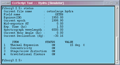
Hydra CTIO presents a terminal window to type commands and send them to the instrument. This command line interface to the Hydra-CTIO instrument gives complete control over the instrument and its functionality. Following is the list with the available commands and a short description of what they do and their arguments.
coldstart [43] - Initialize the motors, find the home positions for the X, Y, and Z axes and resets the encoder to correspond to the center of the focal plate.
home [44] axis - This procedure homes the specified axis and reset the zero point. Available axes are xy, x, w, y, z and gripper. Be aware that homing x, y or w individually *doesn't ensures orthogonality*. Also remember that if x and w are not electrically geared then the gantry can run out of the orthogonal limits.
minit [45] axis - This procedure initialize the specified axis. Available axis are xy, x, y, w, z, gripper. Although you can call x, y or w individually there's only one embedded galil function for initializing the x/y gantry system. This means that no matter you specified x, y or w you will also initialize the other two axes too.
brakes [46] option - Turn the stage brakes on or off. Multiple ways for giving the same order are allowed. To lock the brakes use lock/on/1 as argument. To unlock the brakes use unlock/off/0.
gox [47] x ?vel? ?accel? ?sys? - Move the gripper to the specified position in x leaving the y position the same. Used defaults for the one's that are not supplied in the command line.
goy [48] y ?vel? ?accel? ?sys? - Move the gripper to the specified position in y leaving the x position the same. Used defaults for the one's that are not supplied in the command line.
goxy [49] x y ?vel? ?accel? ?sys? - Move the gripper to the specified position. Used defaults for the one's that aren't supplied in the command line.
gotag [50] tagid - This procedure move the x/y gantry system to the location recorded in the specified tag.
goz [51] z - Move the Z axis to the specified position. Use defaults for missing arguments. The units for position are encoder steps.
gripin [52] - Power up and bring in the gripper.
gripout [53] - This procedure moves the gripper to its stow position. If running under real mode then check for button presence and warn if a button is in the gripper.
tag [54] id ?x? ?y? - This procedure tag the specified location for future reference. It receives as arguments a tag id and an optional coordinate. If only the id is specified by the user, then the current gripper location is taged. The coordinates are x,y sky coordinates.
view [55] name/number ?type? - This procedure let the user view the specified button/object/slit by moving the x/y gantry system to that position. If no type is specified then it will be assumed that the number correspond to a fiber number. Valid names are characters identifying FOPS. Valid type specifiers are "o" for object, "f" for fiber, "s" for slit and "P" for FOPS.
gopen [56] - Open the gripper to its normal open position.
relax [57] - Open the gripper to its relaxed position.
gclose [58] - Close the gripper.
openwide [59] - Open the gripper to its wide open position.
griptest [60] - Test the gripper functionality and return a report.
abump [61] amount direction - Nudge the gripper by the specified amount of arcseconds in the specified cardinal direction. Valid directions are "w", "e", "n" and "s".
bump [62] amount direction - Nudge the gripper by the specified amount of steps in the specified cardinal direction. Valid directions are "w", "e", "n" and "s".
offset [63] dx dy ?vel? ?accel? - Incrementally offset from the current position. Substitute default values for missing arguments.
dropit [64] - Put down a button (if there is one...) at the current location. If the fiber in trouble structure is not empty, calculate and record new information for that fiber.
mark [65] button - This procedure let the user view a button an mark it as the button to be remembered when later you decide to correct the button.
move [66] button x y ?deadzone? - Move a button to the specified location. If the difference beetwen the current location of the button and its target position is smaller than the specified deadzone then the button is assumed to be at the target position.
park [67] button - Move a button to its parked position.
thisis [68] - Handle failures to grab and drop buttons and it helps to identify unknown buttons in the gripper.
ThisIs [69] button - Bring the specified button to the current gripper location. This routine is used to tweak button positions to corrected coordinates interactively.
unstow [70] button - Move the button specified in the argument from its stow position to its park position. If the specified button happens to be the current button in troubles then its trouble condition is cleared.
aload [71] filename - Load a star field. It first looks for it in the directories in environment variables FIBFIELDS and STDFIELDS. If this variables are not defined attempt loading the file using filename as a complete path/filename name.
assign [72] userid button - Attempt to assign the specified object to a button. If the assignment is valid then the button is moved to the object position. The userid corresponds to the id given by the user to each one of the objects of the star field.
configure [73] filename - This procedure configure the star field in file filename.
config1 [74] id x y - This function is much like procedure "configure" except that it takes as an argument a fiber and a coordinate which it passes on to the transition program. This procedure always leave unused fibers alone.
preview [75] first last time - This procedure view the set of objects whoes internal id are beetwen the "first" and "last" specified values. It waits for "time" seconds to get to the next object.
save [76] filename - This procedure save the currently loaded field including tweaks, unassignments, etc been made.
setup field [77] - This command step the astronomet through the field configuration process in order to simplify the instrumental configuration. For a complete description read The Setup Field Command [78].
configmode [79] boolean - This procedure turns the configuration flag on or off. correct Bring the "current" button to the current gripper location. The current button is the last one that was moved or viewed. In some cases, there may not be a current button. This routine is used to tweak button positions to corrected coordinates interactively.
concenmode [80] boolean - Turn the button concentricity correction on/off.
flexmode [81] boolean - Turn the gravitational flexure mapping on or off.
thermmode [82] boolean - Turn the thermal expansion correction on or off.
scalemode [83] boolean - Turn the stage characteristic curve mapping on or off.
lit [84] ?arg arg ...? - This procedure sends its argument list directly to the controller and return just the controller first answer.
ping [85] - This procedure performs a simple test to check communcation towards the Galil Box. It sends a TP command and shows the response. This is the procedure suggested by the vendor to test communications. With good communications you would expect to get a bunch of numbers indicating the current motor positions.
dangle [86] declination - Set the global variable that holds the declination angle. This value is used in flexure calculations.
hangle [87] hourangle - Set the global variable that holds the hour angle. This value is used in flexure calculations.
setcable [88] cable - Set the current cable to the specified cable.
thermval [89] val - Set the instrument temperature to the specified value.
hist [90] - This procedure will open an xterm terminal to show the current session log file.
listdump [91] mode - This procedure when called with argument mode set to "i" dump the iraf file for the currently loaded field and eventually tell the gwc world that it just made it. If called with argument mode set to "c" then dump the currently loaded field to disk and open an xterm running the view program displaying the file contents.
listtag [92] tagid - This procedure will print the coordinates in the tag entry for the specified tag id.
status [93] - Print a summary of the system status. This summary include the current exposure information and the correction flags that are currently working.
where [94] - Return a the encoder positions and corrections.
whereis [95] name/number ?type? - This procedure returns the location of the specified fiber, object, slit or FOPS. The first argument for this procedure can be either an alpha character or an integer. If an alpha character (A, B, C ...) the argument is supposed to be a FOP. If an integer the argument is supposed to be a fiber. A second optional argument can be added to specify what is this integer identifying. Type "f" for fiber, "o" for object and "s" for slit.
purge [96] - Close, compress, and re-open the position archive.
restore [97] - Restore the internal database of button locations from the disk file.
xparked [98] button - This procedure force the software to update a button location to be the parked position.
xstowed [99] button - This procedure force the software to update a buttons location to be the stowed position. If the specified button happens to be the current button in troubles then its trouble condition is cleared.
zdb [100] option - This procedure will zero the database to either stowed or parked position. Set argument position to "parked" to zero to park position and "stowed" to zero to stowed position.
listTI [101] - List the Galil Box Input assignments
listTS [102] - Show the current status of Galil Box switches.
inputchart [103] - Display a window showing the Galil Box inputs.
swchart [104] - Display a window showing the Galil Box switches.
execfile [105] - Source the specified script.
complamp [106] off|tha|etalon|pen|qua|hene - Turn the complams system on/off.
led option ?arg? - This command let the user turn the bank of LEDs on/off and set the current intensity for the light of the LEDs. To turn the LEDs on set argument option to "on". To turn the LEDs off set argument option to "off". To set the current intensity set argument option to "illum" and specify the desired intensity with a number from 1 to 3.
help - Dump the current list of commands and a short description.
plate [107] boolean - Flat/warp the focal plate.
quit [108] - This command exits the application cleanly saving all what has to be saved and leaving the system in a known state.
The field display tool window is the main point of interaction between the user and the instrument. The Field Display Tool allow the user to do from basic things, like commanding the X-Y stages to move, to more high level stuff like configuring a star field using assignment files. It also provide an interface to other systems like the FOPS guider and the comparison lamps.
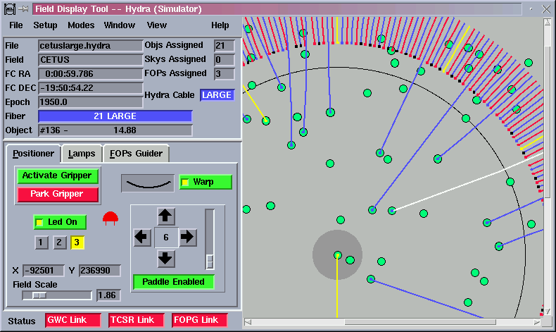
The field display tool include a menu bar, a field info panel, positioner, comparison lamps and FOPS guider control pages, a status bar and a field display.
The menu bar has six options: File, Setup, Modes, Windows, View and Help
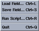
Use the Load Field option to load a star field file. The Hydra-CTIO simulator [109] includes three files of this type that can be used as examples to create your own files. When loaded the objects in the file will be presented in the field display area as springgreen circles, the FOPS as blueviolet circles and the sky positions as lightskyblue squares. Click on the circles and squares to present the name and current assignment of the objects. The related CLI command is aload.
Use the Save Field option to save a star field and you current fiber assignments. Fibers not assigned to objects will be saved as random sky positions. The associated CLI command is save.
Use the Run Script option to run command scripts. The associated CLI command is execfile.
Use the Quit option to exit the application. Before actually exiting the application will prompt the user to decide if he really wants to exit the application. It will also prompt to decide if the X-Y stages have to be left at their transport position (remove from telescope). The user must answer yes to this question only if Hydra is about to be removed from telescope. Finally the user will be prompted to answer yes or no to turn the drives off. We recomend turning the drives off only if you are planning to finish the observing night.
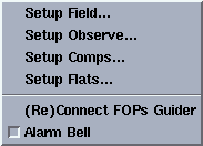
In order to simplify the instrumental configuration, we have created user commands which step the astronomer through the configuration process.
Use this option to configure a star field using a assignment files. When selected a dialog box as the one showed below will come up.
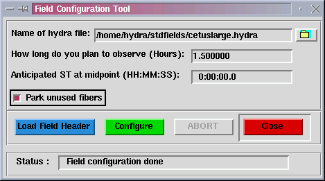
Enter the name of the configuration file you are planning to use in the text entry labeled "Name of hydra file". You can use a complete path or just the name. In this last case the Configuration Tool will search for the requested file at the fields directory. You can also browse to find the configuration file by pressing the button with a folder on it. A file open dialog box will came up and let you select your configuration file.
Press the button labeled "Load Field" to load the configuration file. If the file is not designed for the currently selected fiber cable, a warning message will be given and you will have the opportunity to switch to the cable that your field is designed for. NOTE: This only changes a software flag of cable type. You must still verify that the Bench Spectrograph has the appropriate cable installed. (The cable installed on the Bench Spectrograph should be displayed in the HYDRA-GRAPHICS display.)
Here you will be given the opportunity to modify how long you plan to observe the field in this configuration and what the anticipated midpoint sidereal time will be. Both of these values will be used to fine tune the atmospheric refraction component of the astrometry. If you are rerunning a setup due to a button problem, make sure that you answer these questions in an identical manner as before or the positioner may end up tweaking each and every fiber instead of picking up where it had left off.
You have the option to either park all unused fibers or leave unused fibers where they are as long as they don't interfere with fiber placement by clicking on the check box labeled "Park unused fibers". Leaving them where they are allows such fibers to be flagged as random sky positions and also decreases the configuration overhead since the positioner doesn't have to spend time moving them.
The program will then check certain aspects of the instrument status (plate flat, comps off, rotator at zero degrees), compute the new astrometry, and proceed to move the fibers.
When all fibers have been positioned, the .iraf file will be generated and fiber information will be passed to the CCD for inclusion in the data headers.
NOTE: The instrument is not yet ready to take the observations. You MUST execute the setup observe command.
You can always abort the configuration precedure by pressing the abort button or by typing ^C at the command line. The associated CLI command is setup field.
Use this option to prepare the instrument to start observing. First the gripper LEDs will be turned off, the X-Y stages will move to the field center and the user will be prompt to see if he wants to view any fibers. Answering yes will pop up a window to view the desired fibers by fiber name, by slit position or by assigned object.
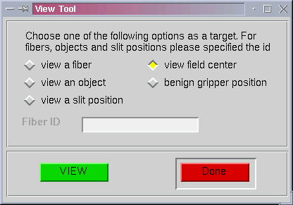
Next either you finish viewing fiber or you answer no to view any fibers, the gripper will be parked. Then you are ready to begin observing. The associated CLI command is setup observe.
Use this option to prepare the instrument to start taking comparison lamps exposures. The gripper LEDs will be turned off and the X-Y stages will be parked. The associated CLI command is setup comps.
Use this option to prepare the instrument to start taking flats. The gripper LEDs will be turned off, the comparison lamps sources will be turned off and the X-Y stages will be parked. The associated CLI command is setup flats.
Use this option to open a connection to the FOPS guider. Not very useful since the automatic recovery procedure was implemented.
Use this option to turn the audible alarm tone on or off.
Use this menu to turn on/off the different types of corrections applied by the model to the x-y coordinates. The thermal expansion correction corrects for thermal expansion in the linear encoders according to vendor specifications. The concentricity correction corrects for the small offset between the center of the button and the fiber. The stage/screw distorsion correction compensate for small distorsion in the stages. The gravitational flexure corrections correct for gravitational effects over the stages.
Use this option to open an xterm window showing the current log file and to open an xterm window showing the currently loaded assignment file.
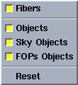
Use this option to show/hide objects, fops, fibers and sky positions at the field display. The Reset option show all the object types in the field.

Use this option to open an xterm window with the available CLI commands.
The status panel consists of a set of labels that show information about the currently loaded star field. The information include header information plus assignment statistics and fiber object cross references.
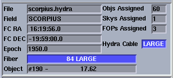
When the user click over an object or a fiber in the field, the Fiber and/or the Obect entry shows the id of the object and its assigned fiber/object.
The positioner tab present a graphic interface to some common user commands to the instrument. Two buttons allow the user to park and activate the gripper. When parked the gripper is moved out of the field and the motor drives are turned off.
Another button allow the user to warp the plate. An animation let the user wait untill the plate is flat or warped before moving fibers.
Another button control the gripper LEDs state and their intensity. There are three available intensities ranging from low to high.
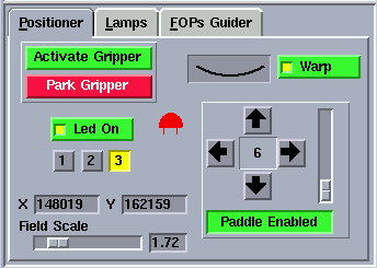
A paddle let the user cruise around using different step sizes. To use the paddle the user must press the button that says "Paddle Disabled". The button will turn green an its text will change to "Paddle Enabled". The arrows keys will change their disable condition to active. Click in the arrows to move the stages. The size of the step in microns can be changed by moving the scale at the right side of the paddle.
The positioner tab also include the x-y coordinates of the cursor while over the field display area and the field display scale control.
The lamps tab allow the user to turn the comparison lamps system on/off and to select the comparison lamps sources.

When no motion is sensed, the status labels are blue and white. When a mechanism is active or moving the status labels blink and the background color goes yellow to reflect the new status. If no status information is available or an error condition is sensed the status labels blink and the background goes red.
The guider bab allow the user to remotely turn the FOPS guider on/off an to enable/disable specific FOPS for guiding.
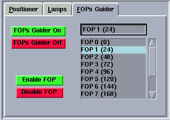
The status bar present the communication links status. The Hydra-CTIO GUI communicates with the FOPS guider through a socket connection and with the TCS through the GWC router. When the communication is working the status labels are green. When the communication links is broken the status labels go red.

Last Modified: May 9, 2000
The graphical display doesn't show an object properly assigned.
This is common symptom that you gave the same number to two or more different objects in your hydra file. Check the number and make sure it is unique.
Hydra error messages start with the word ERROR followed by a sequence of collon separated list of precedure names and explanatory messages. Most of the time is the last part of the message the one that gives more information about what's wrong with the system.
The system returns this error message when the user attempt to execute a Galil box macro while the same Galil macro is under execution. Following are examples of real error messages of this type.
ERROR: gripin: couldn't bring gripper in: gripIn: ColdStart: st_sequence: boxCold: already running or not initialized
ERROR: home: HomeMotors: st_sequence: boxGhome: already running or not initialized
ERROR: move: unresolved: buttonPresent: unable to test: st_sequence: boxIfButt: already running or not initialized
ERROR: tempsense: can't sense temperature: st_sequence: boxTemp: already running or not initialized
The system returns this error messages when the user attempt to execute a Galil box macro while another Galil box macro is under execution. Following are examples of reat error messages of this type.
ERROR: bump: offsetToXY: unresolved: buttonPresent: unable to test: st_sequence: boxIfButt: can't grab the box
ERROR: coldstart: led: st_sequence: boxLed: can't grab the box
ERROR: gripin: couldn't bring gripper in: gripIn: ColdStart: st_sequence: boxCold: can't grab the box
ERROR: gripout: buttonPresent: unable to test: st_sequence: boxIfButt: can't grab the box
ERROR: minit: InitMotors: st_sequence: boxGinit: can't grab the box
ERROR: move: unresolved: buttonPresent: unable to test: st_sequence: boxIfButt: can't grab the box
ERROR: park: buttonPresent: unable to test: st_sequence: boxIfButt: can't grab the box
ERROR: plate: st_sequence: boxIsWarpd: can't grab the box
ERROR: plate: st_sequence: boxPlate: can't grab the box
ERROR: view: buttonPresent: unable to test: st_sequence: boxIfButt: can't grab the box
The system returns this error message when a Galil box macro command has been succesfully written to the serial port, but no response was received in the last 25 seconds. The last under the assumption that no operation takes longer than that. Following are examples of real error messages of this type.
ERROR: brakes: Brakes: st_sequence: boxBrakes: NoResponse
ERROR: coldstart: ColdStart: st_sequence: boxCold: NoResponse
ERROR: coldstart: led: st_sequence: boxLed: NoResponse
ERROR: gox: unresolved: buttonPresent: unable to test: st_sequence: boxIfButt: NoResponse
ERROR: goz: no motion: GoToZ: can't move: st_sequence: boxzgo: NoResponse
ERROR: gripin: couldn't bring gripper in: gripIn: ColdStart: st_sequence: boxCold: NoResponse
ERROR: gripout: buttonPresent: unable to test: st_sequence: boxIfButt: NoResponse
ERROR: home: HomeMotors: st_sequence: boxXYhome: NoResponse
ERROR: home: HomeMotors: st_sequence: boxZhome: NoResponse
ERROR: home: HomeMotors: st_sequence: boxGhome: NoResponse
ERROR: minit: InitMotors: st_sequence: boxGinit: NoResponse
ERROR: minit: InitMotors: st_sequence: boxXYinit: NoResponse
ERROR: minit: InitMotors: st_sequence: boxZinit: NoResponse
ERROR: move: unresolved: buttonPresent: unable to test: st_sequence: boxIfButt: NoResponse
ERROR: move: MoveButt: unknown error: st_sequence: boxMove: NoResponse
ERROR: openwide: OpenWide: st_sequence: boxOpen: NoResponse
ERROR: park: ParkButt: MoveButt: unknown error: st_sequence: boxMove: NoResponse
ERROR: park: buttonPresent: unable to test: st_sequence: boxIfButt: NoResponse
ERROR: plate: st_sequence: boxPlate: NoResponse
ERROR: view: buttonPresent: unable to test: st_sequence: boxIfButt: NoResponse
ERROR: view: buttonview: ViewButt: GoToXY: can't move: st_sequence: boxxygo: NoResponse
The error message above may indicate problems in the serial link between Hydra Instrument and its host computer.
Check that the Galil Box is up and running and that the serial link is OK. Try the ping command [85] to test the link. If it works then the Galil Box might be in error condition. Try cycling the power.
This error message indicates that the drive power is off. Following are examples of real error messages of this type.
ERROR: gripout: gripOut: no xy motion: GoToXY: can't move: st_sequence: boxxygo: NoDrive
ERROR: minit: InitMotors: st_sequence: boxZinit: NoDrivePower
ERROR: view: buttonview: ViewButt: GoToXY: can't move: st_sequence: boxxygo: NoDrive
This error message indicates that the Z motor was not properly initialize during a cold start sequence (i.e. coldstart [111] and gripin [52] commands). During a cold start sequence the Z motor is powered up and then initialized to its zero point. Following are examples of real error messages of this type.
ERROR: coldstart: ColdStart: st_sequence: boxCold: NoZInit
ERROR: gripin: couldn't bring gripper in: gripIn: ColdStart: st_sequence: boxCold: NoZInit
To figure out what exactly caused the problem try manually initializing the motor using the minit z command [45] and the home z command [44]. Then look for the new error messages in this trouble shooting guide.
This error message indicates that the motor was unable to find the fiducial point. The motor is then probably at one of its limits. Following are examples of real error messages of this type.
ERROR: gripout: gripOut: HomeMotors: st_sequence: boxZhome: NoHome
ERROR: home: HomeMotors: st_sequence: boxZhome: NoHome
Unfortunately often this failure to find the fiducial hangs the Galil built in macro to find the zero point and prevent the box from answering to further command macro requests. Below is a crude procedure to try to clear this fault.
If the above doesn't work you might have to check hardware issues like drive power, limit switches, optical switch, etc.
This error message indicates that at least one of the following safety intelock signals has been activated: FSA interlocks, orthogonality switch, forward and reverse X-Y limits. Following are examples of real error messages of this type.
ERROR: goxy: no motion: GoToXY: can't move: st_sequence: boxxygo: FsaOrthoRFL2
ERROR: gripout: gripOut: no xy motion: GoToXY: can't move: st_sequence: boxxygo: FsaOrthoRFL2
ERROR: view: buttonview: ViewButt: GoToXY: can't move: st_sequence: boxxygo: FsaOrthoRFL2
Each of the interlocks mentioned above are AND gated before input to the Galil Box. So when the this error message occurs all three possible causes has to be checked, that is, check that the FSA is properly closed, check that the second forward and reverse limits are clear and check that the system is orthogonal. Read the listTI command [101] documentation since it can be of great help when dealing withi problem.
This error message indicates that the stages had not been initialized. Use the coldstart command [111] to initialize the system. Following are examples of real error messages of this type.
ERROR: goxy: no motion: GoToXY: can't move: st_sequence: boxxygo: Inhibited
ERROR: gripout: gripOut: no xy motion: GoToXY: can't move: st_sequence: boxxygo: Inhibited
ERROR: view: buttonview: ViewButt: GoToXY: can't move: st_sequence: boxxygo: Inhibited
This error message appears when the system has been commanded to move while the gripper is below its home position. The home position for the gripper is high enough to clear the fibers on the field as well as the fiber slots. Following are examples of real error messages of this type.
ERROR: dropit: releaseHere: DisposeButt: GoToXY: can't move: st_sequence: boxxygo: BelowHome
ERROR: park: ParkButt: DisposeButt: GoToXY: can't move: st_sequence: boxxygo: BelowHome
ERROR: view: buttonview: ViewButt: GoToXY: can't move: st_sequence: boxxygo: BelowHome
To clear this problem move the gripper up at least to its home position. In order to do that you can either home the gripper with the coldstart command [111] or move it with the goz command [51] and a positive value.
This error message indicates that an error ocurred during the initialization of the x and y motors. Following are examples of real error messages of this type.
ERROR: home: HomeMotors: st_sequence: boxXYhome: AxisFailure
Use the listTI command [101] to figure out which of the motors is causing the problem and why.
This message indicates that the system has found a button in the gripper at the moment of initialization. You may have to follow a recovery procedure to drop the button before initializing the system. Following are examples of real error messages of this type.
ERROR: coldstart: ColdStart: st_sequence: boxCold: ButtonOnInit
ERROR: gripin: couldn't bring gripper in: gripIn: ColdStart: st_sequence: boxCold: ButtonOnInit
The recovery procedure starts by initializing the gripper motor and the Z axis motor using the minit command [45] and then the home command [44] for each axis.
For example to initialize the axis:
Fiborg3.2.5> minit gripper
Fiborg3.2.5> home gripper
Fiborg3.2.5> minit z
Fiborg3.2.5> home z
The second step is to drop the button by using the dropit command. It may be necessary to issue the command several times before the system
drop the button. If no success open the gripper to its wide open position and try removing the button from the gripper jaws manually.
This message appear when the motor is not able to finish its motion. Try the listTI command [101] for more diagnosis information. Following are examples of real error messages of this type.
ERROR: goz: no motion: GoToZ: can't move: st_sequence: boxzgo: NoMotion
This message appear when a the system has been ordered to move the stages while the stages are at their park position. Following are examples of real error messages of this type.
ERROR: bump: offsetToXY: GoToXY: gripper is disabled, use gripin to activate
ERROR: goxy: no motion: GoToXY: gripper is disabled, use gripin to activate
ERROR: move: MoveButt: gripper is disabled, use gripin to activate
ERROR: park: ParkButt: MoveButt: gripper is disabled, use gripin to activate
ERROR: view: buttonview: ViewButt: GoToXY: gripper is disabled, use gripin to activate
Activate the gripper either by using the GUI button or typing the gripin command [52]
This message appear if the user has tried to activate the gripper too soon after parking it. For some unknown reason the motor drives have to rest a few seconds after been turned off to prevent the Galil Box to run into a fault condition. Following are examples of real error messages of this type.
ERROR: coldstart: ColdStart: please wait a few seconds and try again
ERROR: gripin: couldn't bring gripper in: ColdStart: please wait a few seconds and try again
This message appear when the user tries to move the gripper to a non valid position. Following are examples of real error messages of this type.
ERROR: bump: offsetToXY: GoToXY: target is beyond X-Y limits
This message tell the user he has tried to move a fiber that has been marked as "non existant" in the concentricities [112] configuration file. Following are examples of real error messages of this type.
ERROR: configure: mqu_orderMoves: ERROR: park: ParkButt: MoveButt: fiber #102 doesn't physically exists...
ERROR: configure: mqu_orderMoves: ERROR: physmove: MoveButt: fiber #2 doesn't physically exists...
ERROR: configure: orderMoves: ERROR: physmove: MoveButt: fiber #2 doesn't physically exists...
ERROR: fieldsetup2: ERROR: configure: mqu_orderMoves: ERROR: park: ParkButt: MoveButt: fiber #232 doesn't physically exists...
ERROR: fieldsetup2: ERROR: configure: mqu_orderMoves: ERROR: physmove: MoveButt: fiber #232 doesn't physically exists...
ERROR: move: MoveButt: fiber #10 doesn't physically exists...
ERROR: park: ParkButt: MoveButt: fiber #102 doesn't physically exists...
Check the concentricities [112] configuration file for more information about the fiber.
This error message tell the user he has tried to stowed a fiber that is not actually stowed, that is, is not at its fiducial position in the plate. Following are examples of real error messages of this type.
ERROR: unstow: Unstow: button 249 is not stowed
This message appear when the user tries to move a fiber with the plate at its warp position. Following are examples of real error messages of this type.
ERROR: configure: can't move with plate warped
ERROR: move: can't move with plate warped
ERROR: park: can't move with plate warped
Use either the GUI button or the plate command [107] to unwarp the plate.
This message appear when the user tries to move a fiber to a non-valid position. The actual reason why the target position is not valid can be found at the xterm window from which hydractio was launched. Following are examples of real error messages of this type.
ERROR: configure: mqu_orderMoves: ERROR: physmove: invalid move requested for button #207
ERROR: configure: orderMoves: ERROR: physmove: invalid move requested for button #159
ERROR: fieldsetup2: ERROR: configure: mqu_orderMoves: ERROR: physmove: invalid move requested for button #88
ERROR: move: invalid move requested for button #0
This message tell the user that the position that the known position of the fiber is out of bounder. Following are examples of real error messages of this type.
ERROR: configure: mqu_orderMoves: ERROR: park: ParkButt: MoveButt: it's not safe to grab button at current location
ERROR: fieldsetup2: ERROR: configure: mqu_orderMoves: ERROR: park: ParkButt: MoveButt: it's not safe to grab button at current location
This is a very unusual error message and may be an indication that the Galil Box variables that are set the first time the application starts up has been corrupted some how or the result of incorrect use of either thisis [68] or ThisIs [69] recovery commands.
This message tell the user that the system failed in grabing the specified button. Following are examples of real error messages of this type.
ERROR: configure: mqu_orderMoves: ERROR: park: ParkButt: MoveButt: couldn't pick up button 1
ERROR: configure: mqu_orderMoves: ERROR: physmove: MoveButt: couldn't pick up button 101
ERROR: configure: orderMoves: ERROR: park: ParkButt: MoveButt: couldn't pick up button 159
ERROR: configure: orderMoves: ERROR: physmove: MoveButt: couldn't pick up button 247
ERROR: fieldsetup2: ERROR: configure: mqu_orderMoves: ERROR: park: ParkButt: MoveButt: couldn't pick up button 0
ERROR: fieldsetup2: ERROR: configure: mqu_orderMoves: ERROR: physmove: MoveButt: couldn't pick up button 7
ERROR: move: MoveButt: couldn't pick up button 0
ERROR: park: ParkButt: MoveButt: couldn't pick up button 84
To actually pick up the button we recommend using the thisis [68] or ThisIs [69] command to correct the known coordinates of the software. You will have to cruise around and center the gripper on top of the button and then issue one of the two commands. Then park the button.
This message indicate that the button was lost during the move. This is a very dangerous situation sice is not possible to know were the button was left. Following are examples of real error messages of this type.
ERROR: configure: orderMoves: ERROR: physmove: MoveButt: gripper has no button to drop
ERROR: fieldsetup2: ERROR: configure: mqu_orderMoves: ERROR: park: ParkButt: MoveButt: gripper has no button to drop
ERROR: fieldsetup2: ERROR: configure: mqu_orderMoves: ERROR: physmove: MoveButt: gripper has no button to drop
ERROR: move: MoveButt: gripper has no button to drop
ERROR: park: ParkButt: MoveButt: gripper has no button to drop
You can use the gripper camera two see if you can find the button and then update its last known coordinates to its current position with the ThisIs command [69] . The other way to go is to manually stow the fiber and then tell the software with the xstowed command [99] that the fiber is now stowed.
This message tell the user that the gripper still has the button in the gripper after trying to drop it at its target position. Following are examples of real error messages of this type.
ERROR: configure: mqu_orderMoves: ERROR: park: ParkButt: MoveButt: couldn't drop button 88
ERROR: configure: mqu_orderMoves: ERROR: physmove: MoveButt: couldn't drop button 174
ERROR: dropit: releaseHere: DisposeButt: DropButt: couldn't drop button!
ERROR: move: MoveButt: couldn't drop button 170
ERROR: park: ParkButt: DisposeButt: DropButt: couldn't drop button!
ERROR: park: ParkButt: MoveButt: couldn't drop button 103
Try releasing the fiber using the dropit command [64]. This command will try to cleanly release the fiber at the current gripper position. Try it several times, sometimes takes more than one try to release the offending fiber.
If the above doesn't work you can still try opening the gripper jaws to their open wide position using the openwide command [59]. This command will open the jaws more than usual hopefully releasing the button. If not then try releasing it manually.
This message tell the user that there is no button in the gripper to drop.
This message tell the user that the software has a record of another fiber at the current gripper position when using the thisis command [68] . This prevents from giving a button the coordinates of another button.
ERROR: ... : fiber in jaws - this message appear when trying to park the gripper while holding a button in the gripper. Following is an example of this type of message.
ERROR: gripout: fiber in jaws
This message tell the user that te system won't move any other fiber until he resolves the problem with a lost fiber. Following is an example of this type of message.
ERROR: configure: mqu_orderMoves: ERROR: physmove: can't move button 0 with 168 in transit
You will have to find the lost fiber and then update its current location with the thisis [68] or ThisIs [69] command. Only then you will be able to continue moving fibers. Not knowing the lost fiber position can result in fiber collisions.
The read temperature value is out of range. You can override the read value by manually entering the temperature value using the themval command [89]. Following are some examples of this type of message.
ERROR: tempsense: can't set current temperature: ERROR: thermval: temperature is to large/small
This message tell the user that it was not possible for the software to do a transition from its current configuration to the one specified by the assignment file. The error message now includes information about the offending fiber. Following are examples of real error messages of this type.
ERROR: configure: mqu_orderMoves: ERROR: transition: unable to do the transition. Please check your assignment file for invalid moves.
ERROR: transition: unable to do the transition. Please check your assignment file for invalid moves.
The short way to solve this problem is to comment out the line in your assignments file containing the offending fiber assignment. The long way is to run hydraassign and get new assignments for the objects in the file.
The init file astroparams [113] is corrupted or the environment variable that holds the path to the file is undefined. Check your environment for the ASTROPARAMS environment variable, check you read permissions to the astroparams file and check that the file actually exists.
The init file systemparams [114] is corrupted or the environment variable that holds the path to the file is undefined. Check your environment for the SYSTEMPARAMS environment variable, check you read permissions to the systemparams file and check that the file actually exists.
the transition program was unable to open the script containing fiber moves.
ERROR: configure: mqu_orderMoves: ERROR: transition: hydra file "parkall" not found.
ERROR: transition: hydra file "parkall" not found.
The transition program was unable to find the plate coordinates file created by the astrometry program. Following are examples of this type of message.
ERROR: configure: mqu_orderMoves: ERROR: transition: transition couldn't find file: "GM.1.out1.hydra.coords"
ERROR: transition: transition couldn't find file: "GM.1.out1.hydra.coords"
Check for error messages about the astrometry program.
the scpecified file name doesn't exist. Following are examples of this type of message.
ERROR: fieldsetup2: ERROR: aload: file /home/hydra/fields/GM.out2.hydra doesn't exists
The user interrupt the script execution by typing ^C. Following are examples of this type of message.
ERROR: User interrupt while sourcing largecircle
This message tell the user that no connection was opened to the FOPS guider. Check the ethernet connection and check that the FOPS guider program is actually running.
This message tell the user that the program failed to send the command to the FOPS guider. Check the ethernet connection and check that the FOPS guider program is actually running.
This message tell the user that the program failed to read the command response coming from the FOPS guider. Check the ethernet connection and check that the FOPS guider program is actually running.
Last Modified: May 9, 2000
The measurement of concentricities has to be made off telescope probably at the Coude Room. The minimal setup required to measure the concentricities includes, besides Hydra, a video monitor, an ICCD controller, a video cursor, a light source and the Hydra Laptop (or the Hydra PC). The video monitor plus the ICCD controller display the video signal from the gripper camera. The light source is used to illuminate the fibers from behind. And the Laptop controls the instrument. When illuminating the fibers environmental light has shown to be sufficient for the small and large fibers. To illuminate the FOPS it's not necessary to remove the FOPS camera. Removing the filter in front of the camera will allow you to introduce enough light through the space left by the filter.
If you are using the Hydra Laptop to control the instrument during this procedure you better be sure that the "CurrentLocations" and "statusFile" are not different from the ones in ctioa6 (Hydra PC). Copying this files from ctioa6 to the laptop will ensures that the software knows exactly where the fibers are. For example if the Ethernet connection is available, typing the following commands in a shell window will do it for you. Don't forget to login as "hydra".
% cd Hydra/data/status
% rcp ctioa6:/home/hercules/Hydra/data/status/CurrentLocations .
% rcp ctioa6:/home/hercules/Hydra/data/statuc/statusFile .
Now you can start "hydractio" or "hydractio-comm" if you don't want to communicate with the TCS and FOPS Guider systems (this will be often the case).
The canonical procedure is first to put the fibers in a circle. There is a script that can do this job for you. For example, if you are measuring the concentricities for the small fibers type at the CLI/Script Tool command line:
Fiborg3.2.0> execfile configsmallcircle
After it finishes you can execute the script to actually measure the offset between the button position and the fiber position for every fiber. Don't forget to check that your light source is illuminating the fibers evenly before executing the script. What the script does is to go fiber after fiber grabbing its current position, allowing you to correct the position by offsetting the gripper and grabbing the new position. The idea is to use a video reference (video cursor) to center, by moving the gripper, the light beam coming from the fiber and use the offset between the original (button position) and final position (fiber position) to calculate the concentricity correction for that particular fiber. You should repeat the process a minimum of three times (five is a good number of repetitions), that is parking all the fibers, putting them back in a circle and grabbing the corrections. Make sure you also do FOPS concentricities measurements interleaved with the small or large concentricities measurements. The FOPS serve as the zero point correction. It is recommended to do all the fibers (small, large and FOPS) with the same TV setup just to ensure that they are all on the same zero point. All the recorded positions are kept in the log file of the current session.
For example, if you want to record concentricity data for the small fibers you should type at the CLI prompt:
Fiborg3.2.0> execfile meassmall
The gripper will move to the first small fiber and will wait for you to move the gripper. You can use the arrow buttons in the "Field Display Tool" window or the keyboard by typing "h, j, k, l" (make sure the mouse cursor is on top of the "Field Display Tool" window) to offset the gripper. You can change the size of the step by moving the red slider in the field display or by pressing a key from 1 to 9. After you finish with the first fiber type "q" or press the "Enabled" green button. At this moment the "Enabled" button will go red, the gripper will move to the second small fiber and the "Enabled" button will go green again. Repeat the process above until you finish all the small fibers.
After you finish logging the concentricities raw data you can use the "concenctio" program to generate a new concentricities file. [112] This program lives in /home/hydra/src/concenct. First you'll have to copy the old concentricities files to that directory plus the log file(s) containing the raw data. The old concentricities file will be used as a template to produce the new file. If the name of your current concentricities file is different than "concentricities" you will have to rename it as "concentricities". Then run the program to generate the new concentricities file. The name of the new file will be "nconcentricities". For example, to generate a new concentricities file from the current "concentricities" file plus the "hydra.currentLog" log file you should do:
% cd /home/hydra/src/concenct
% cp /home/hydra/Hydra/data/inits/concentricities .
% cp /home/hydra/fiblogs/hydra.currentLog .
% concen
Enter the name of the log file: hydra.currentLog
Small Concentricities
Group 1 Average is X= 0.000000 Y= 0.000000 for 135 measurements
Another file to read? (y or n): n
ave x = 0.000000, ave y = 0.000000, sdev x = 0.000000, sdev y = 0.000000
ave r = 0.000000, sdev r = 0.000000
var = 0.000000
var = 0.000000
var = 0.000000
ave x = 0.000000, ave y = 0.000000, sdev x = 0.000000, sdev y = 0.000000
ave r = 0.000000, sdev r = 0.000000
var = 0.000000
var = 0.000000
var = 0.000000
.
.
.
ave x = 0.000000, ave y = 0.000000, sdev x = 0.000000, sdev y = 0.000000
ave r = 0.000000, sdev r = 0.000000
var = 0.000000
var = 0.000000
var = 0.000000
%
If the data is contained in more than one log file, then copy all the log files to the concenct directory and answer yes to the question "Another file to read? (y or n):". The program will prompt you for the name of the second file, third file, etc.
When you run the program, make sure you also enter the large fiber and FOPS concentricity measurements (either a new set or old data took previously) to make sure that the zero point correction is handled appropriately.
Besides the nconcentricities file there are four other output files: raw.dat, ave.dat, con.dat and plot.macro. "plot.macro" is a supermongo script to generate individual plots for the concentricity measurement for each fiber. It uses the "ave.dat" and "raw.dat" files. File "con.dat" is for diagnostic value in case something looks strange. For example, to print the concentricity measurement plots:
% sm (sm is available in solaris and sunos workstations)
Hello hydra, please give me a command
: macro read plot.macro
: device postlandfile plotset1.ps
: plotset1
: device postlandfile plotset2.ps
: plotset2
: device postlandfile plotset3.ps
: plotset3
: device postlandfile plotset4.ps
: plotset4
: device postlandfile plotset5.ps
: plotset5
: device postlandfile plotset6.ps
: plotset6
Remember to place a comment in the header of the new concentricities file and to increment its version number. Then copy the new concentricities files to its final location at the Hydra PC and test at the telescope by configuring a standard field.
Last Modified: April 27, 2000
Before you can download code, you need to have the appropriate hardware and software configurations. Various switches and software items need to be configured. These are discussed below for both the host machine and the Galil Box.
a) Host Machine
The easiest way to download the code is to use the "Editor Tool" provided with the Visual Basic Tool. In order to use this software you will need your host machine to be running under Windows95 and the Visual Basic Tool installed.
b) Galil Box
While a comprehensive discussion of the Galil DMC-1500 is ledt to the Galil User Manual, a few pointers are given below.
In order to be able to do anything with the box, you have to be able to talk to it. To that end, a cable and the correct switch settings are required. No other hardware is necessary to talk to the box. Notice the little set of dip switches next to the serial ports on the black box. Set them as follows:
| switch # | Name | Position |
| 1 | MRST | OFF |
| 2 | 1200 | OFF |
| 3 | 9600 | OFF |
| 4 | 19.2k | OFF |
| 5 | HSHK | OFF |
This will set up things up for a baudrate of 9600 with no hardware handshake.
Now that you have the right hardware and software configuration you can start the Visual Basic Tool and get ready to download the code.
Start the Visual Basic Tool application and press the button labeled "Source Edit". The Editor Tool window will appear. Use the file directory window to browse for your makefile file. The Editor Tool use this file to load the files containing the code you are planning to download. This is a simple text file with a newline separated list of file names. If you are downloading the Galil Embedded Code [115] that file is "makefile.mak". It includes seven files: buttmove.g, coldstrt.g, errors.g, gripops.g, main.g, periphio.g and xyops.g.
Choose the makefile by clicking on it. The contents of the file will be showed in the "Make File Contents" entry. Here the Editor Tool gives you the opportunity to check the code in the files you just loaded before you attempt to make a download. Remember that each time you make a download the current code is lost. Click a file name in the "Make File Contents" box and the source code and declared variables will be showed.
The final step is to download the code into the Galil. Press the button labeled "Download all files" to download the code. The download will take approximately 25 seconds. If everything went O.K. then a dialog box should pop up saying "Download OK".
Last Modified: April 27, 2000
Software binaries are available to run under Linux and Solaris. The latest versions will be found in hydrasimLinux [2] for Linux and in hydrasimSolaris [1] for Solaris. Both versions can also be found in the Tucson mirror of the CTIO ftp site [116] (updated nightly). Current version of the software is 4.0.2.
You will probably also want to download the the documentation file hydraassign.ps [37]. Thanks to Phil Massey for providing the documentation and software for the Hydra-CTIO version of hydraassign [42].
First, be sure you are running the c-shell or one of its derivatives (e.g. tsch). If you are running the bash shell, you can change to the c-shell using the command chsh -s /bin/csh Put the tar file in your home directory, change to your home directory and then
gunzip hydrasimLinux.tar.gz
tar -xf hydrasimLinux.tar
uncompress hydrasimSolaris.tar.Z
tar -xf hydrasimSolaris.tar
Now change to subdirectory "/Hydra/bin" and execute "~/install.org". This is a script that will create three sub-directories (fiblogs, fields & stdfields) in your home directory. Copy the file "~/Hydra/bin/sample.fiborg" to .fiborg in your home directory as well. Then include in the "set path" command of either your ".login" or ".cshrc" file the following path:
~/Hydra/bin
Also, add the folowing line to your .login or .cshrc file to source the .fiborg and set the environment:
source ~/.fiborg
Log out and back in to allow the new path to be activated or type "source ~/.login" (or source ~/.cshrc or whatever is your particular rc file). If you chose not to decompress and de-tar the downloaded file in your home directory change variable FIBHOME in file ".fiborg" to reflect the new location of the software as well as the bin path for the "set path" command.
Two windows will appear. One is a simple command line window (CLI/Script Tool window) and the other is a window showing a graphical representation of the fibers and the focal plate. It also includes various information about the current star field and status. The terminal window used to launch the program will be used as a console.
Last modified: October 17, 2001
This program lets you define the screen positions for the FOPS. The program runs in the same vme pizza box where the hydra guider does.
First edit the boot parameters by booting the computer and stopping the countdown sequence (to reboot type reboot at the prompt or Ctrl+X). To edit the boot parameters type c and then press enter, as follows:
[VxWorks Boot]: c
In response, the boot program prompts you for each parameter. Change the startup script field to "/tftpboot/align.cmd":
startup script (s) : /tftpboot/align.cmd
That will download the right binary and will setup things to run the alignment program.
To run the FOPS alignment program call the function AlignFops from the vxWorks shell. When the program starts you will have the X,Y,Z and Mode information at the top of the screen and a box in the center of the screen. To move the box use the arrow keys on the numeric keypad. Make sure that
NUMLOCK is on.
The <tab> key will increment the step size that the box moves with each key stroke. The range is from 1 pixel per key to 20 in steps of 5. It will be clear how it works once you test it out.
Make sure you are in Mode 0. This is done with the ] key. Move the box so that the first fop you want to align is centered in it. Once you have the FOP centered in the box record the X, and Y values. These are the ROI starting coordinates for this FOP.
Now switch to mode 1, (the [ key). Again, using the arrow keys on the numeric keypad move the aligment dot to the center of each FOP fiber and record the X,Y coordinates. The Z value is displayed to aid in choosing the center of the fiber.
Now switch back to mode 0 (the ] key). Do this for each FOP.
Once you collect all of the data you need to put it into the hydra.ini file in the proper format.
It is important to collect fiber information from each FOP in the same order. I usually start with the top most fiber and proceed clockwise ending with the center fiber.
Once you have a good INI file you can check the alignment by loading the guider code and calling the function regFiber(0). This will display the alignment boxes around each fiber of
each FOP. To turn these off call regFiber(3).
Some debug information that you can display is very helpful. Once the guider code is running, in the vxWorks shell you can set nDebugLevel1, to the value '1'. This will start the debugging output. Setting it equal to 0 will turn it off.
nDebugLevel1 will give the (for each FOP)
FopID
Fiber #
Fiber Mean Intensity
Fiber Mean Intensity - Background,
Sky level,
Frame bias value,
Number of pixels in fiber ROI
Sum of the pixels in the fiber ROI
Last Modified: October 17, 2001
At the VxWorks prompt type "Guide". You will notice that the FOPS monitor will flash and then a bunch of messages will be printed to the terminal output:
-> Guide
Before guiding you have to activate the Fops you want to use. You can activate the FOPS by sending the command from the Hydra-CTIO gui or by typing a command at the VxWorks shell prompt.
In the first case select the fiber from the list and press the green button labeled "Enable FOPS".
In the second case just type chgFop(fop#, type, state), where:
fop# is the fop number from 0 to 11.
type is 1 for GUIDE, 2 for SKY and 3 for MONITOR.
state is 1 for active and 2 for inactive.
For example to activate FOPS 6 as a monitor FOPS type:
-> chgFop(6, 3, 1)
Finally to start guiding press the green button labeled "Guider On" or type at the VxWorks shell prompt:
-> GuiderOn
To stop guiding type:
-> GuiderOff
Last Modified: March 11, 1999| Contents: | |
| 1. | Software Code |
| 2. | Starting The Program |
| 3. | Hydra GUI |
| 3.1 Menu Bar | |
| 3.2 Status Panel | |
| 3.3 Control Panel | |
| 3.4 Status Bar | |
| 4. | GWC Status Variables |
| 5. | Trouble Shooting |
The Hydra Spectrograph GUI software lives in /usr/local/Bench4m. The structure of the directory tree is as follows:
The Hydra spectrograph GUI consists of an extended TCL/TK interpreter plus a set of TCL/TK scripts that build the functionality required by the application. The extended TCL/TK interpreter lives at sub directory "src". Support is provided for compiling the interpreter under Linux, SunOs and Solaris. The TCL/TK scripts live at sub directory lib/bench4m and lib/common.
Open an xterm window and type start_bench4m to start the program. This start up shell script will search your home directory for file .bench4mrc to set the environment before running. If not found it will look for the default version of that file at /usr/local/Bench4m/bin for bench4mrc.
Following is an example of that file:
#-------------------------------------------------------
#!/bin/csh
# Environment variables for the hydra spectrograph gui program
#
# modification history
# --------------------
# 01a 04apr2000, rcr - Created
# Bench 4m environment
setenv BENCH4MHOME /usr/local/Bench4m
# The TCL/TK package libraries
setenv TCL_LIBRARY $BENCH4MHOME/share/lib/tcl8.0
setenv TK_LIBRARY $BENCH4MHOME/share/lib/tk8.0
# The MPG_ROUTER variable designates the name of the host in which
# the router run. When not defined the the mpg router is supposed
# to be running in indus.tuc.noao.edu.
setenv MPG_ROUTER ctioa1
# The variable MPG_ROUTER_PORT designates the port in which the mpg
# router is listening for incoming connections. The default value
# for this variable is 1 plus the the wiyn router port (2345).
setenv MPG_ROUTER_PORT 2347
# Directory containing configuration files
setenv BENCH4MCONF $BENCH4MHOME/config
# Serial port to connect to
setenv BENCH4MSPORT /dev/ttya
# Others
#setenv PATH $PATH":/usr/local/bench4m/bin"
#setenv LD_LIBRARY_PATH /local/X11R5/lib:$LD_LIBRARY_PATH
#------------------------------------------------------
The program also use three configuration files that live at /usr/local/bench4m/config: gratings.conf, bench4m.ini and filters.ini.
gratings.conf - text file containing grating parameters. Following is an example of this file:
| -------------------------------------------------------------- | |||||||
| # CTIO Hydra Bench Spectrograph gratings parameters. | |||||||
| # Name | l/mm | Blaze | Wrange | Disp | gr_0 | gr_fdg | incl_0 |
| KPGL3 | 527 | 5500 | 3417 | 1.16 | -0.3 | 0.988 | 0.0 |
| KPGL1 | 632 | 4200 | 2872 | 1.02 | -0.491 | 0.988 | 0.0 |
| KPGLF | 632 | 8200 | 2872 | 1.01 | -0.30 | 0.988 | 0.0 |
| G450 | 632 | 11000 | 2872 | 0.47 | -0.33 | 0.988 | 0.0 |
| KPGLD | 790 | 8500 | 2290 | 0.79 | -0.27 | 0.988 | 0.0 |
| KPGLG | 860 | 11000 | 2101 | 0.68 | -0.3 | 0.988 | 0.0 |
| G380 | 1200 | 8000 | 1563 | 0.48 | -0.3 | 0.988 | 0.0 |
| Echelle | 316 | 56120 | 2888/ | 0.94/n | -0.1 | 0.988 | 0.0 |
| -------------------------------------------------------------- | |||||||
name - a label for the grating
l/mm - number of lines per millimeter
Blaze - self explanatory
Wrange - wavelength range
Disp -
gr_0 - grating angle value for order 0
gr_fdg -
incl_0 - fiber head assembly angle for
bench4m.ini - text file containing the last grating and grating order used. There is a user version of this file called ".bench4m.ini". When the user exits the application the grating and the grating order are saved to this file at the home directory.
filters.ini - text file containing the last filter labels used. There is a user version of this file called ".filters.ini". When the user exits the application the filter labels he defined are saved to this file at the home directory.
The Hydra Spectrograph GUI (shown below) is the front end which controls the motors on the Hydra Bench Spectrograph. The GUI connects to a "Smart Motor Controller" (SMC) which controls each of the motors via a serial line through which status information and movement commands are sent.
The GUI also connects to the so-called "GWC" router which publishes the status of the various motors and switches. This allows Arcon to build header information during image acquisition.
At the top of the GUI is a menu bar with four pop-up menus: Setup, Windows, Options and Help.
Clicking on "Setup" gives you three options:
Use the "Load Grating" option to select the desired grating. The gratings database is loaded from a text file called "gratings.conf". This file can be manually edited to add new gratings. This file is loaded when the application starts and every time the "Gratings" dialog box is opened.
Use this option also to set the current grating order. The current grating and the current grating order appear in the GUI title bar.
This dialog box will also appear when you press the left mouse button over the "Grating" entry on the main GUI. The selected grating and the grating order will be saved in the initializstion file (bench4m.ini) whenever you exit the application.
This option allows you to view the current grating specifications. The user must select a grating using "Load Grating" before using this option. The data presented in this box is read from the grating database each time "Load Grating" is used.
Note: Grating parameters may not be altered in this window. They can only be changed by manually editing the gratings.conf file.
The "Filter" option permits the user to label the installed filters with names. Labeling the filters will allow the program to publish the filter names through the GWC router. The user names will also be used to label the filter control buttons on the GUI.
The filter labels you are saved every time the application is exited.
The "Windows Option on the GUI menu offers a single option: "Terminal". This opens a terminal window allowing one to manually send commands to the SMC. The user should not normally have any need to use this option.
If commands must be sent manually to the SMC, read the following document explaining the syntax and function of SMC commands [117]. This is usually only done for testing and diagnosing equipment failures.
The "Options" menu presents a single option: "Alarm Bell". Use this option to activate/deactivate a bell tone that warns the user that the link to the GWC router is not functioning.
The status panel consists of a set of labels that show the current status of the spectrographs motors and switches. When no motion is sensed, the status labels are blue and white. When a mechanism is active or moving the status labels blink and the background color goes yellow to reflect the new status. If no status information is available or an error condition is sensed the status labels blink and the background goes red.
The control panel consists of a set of widget clusters that group some common functionality.
Four clusters are present: grating control, fiber mount focus control, shutter/newall control and
filter wheel control.
Use the grating control panel to set the grating tilt angle the inclination of fibers angle. To set this values the user must load a grating with the "Load Grating" option first.
The user typically enters a wave length and press return to calculate the proper grating tilt angle and inclination angle. To actually move the mechanisms the user must select "Set Grating and Inclination Angles" from the "Commands" menu button.
Use the fiber mount focus control panel to set the focus distance. The user typically enters a focus value and press return to actually move the focus mechanism.
Use the shutter/newall control panel to set the shutter/newall position. The actions taken depend on whether control of the shutter comes from the SMC or Arcon.
When the SMC is in control, the actions taken are immediate and direct. The shutter is a large rotating disc. If you ask for it to be open or closed, it does exactly what you expect. When you ask for "upper" or "lower" position, it moves to a positions with the upper or lower half of the aperture covered.
When control over the shutter is transferred to Arcon, if "Newall normal" has been selected, Arcon will open the shutter fully when an exposure begins. If "Newall upper" or "lower" is selected, during the exposure the respective half the aperture is left covered. At all other times the shutter remains fully closed.
Use the filter control panel to set the filter wheel position and to set the LEDs intensity.
So far the status bar has a single widget that presents the status of the GWC link. When the GWC link brakes the widget goes blinking and if the "Alarm Bell" option is set, a tone will be heard.
The status information collected by the application is published by the GWC router to other applications that use it (i.e icsInfo). Following are the data streams that the application defines to publish its data. Client applications can subscribe to this data through the GWC router.
bench4m.main.grat - grating angle (degrees)
bench4m.main.fiber - fiber mount focus
bench4m.main.filter - filter position
bench4m.main.shutter - Shutter position
bench4m.main.newall - Newal mask position
bench4m.main.led - LED status (on/off)
bench4m.main.incli - fiber line inclination
Check that the GWC router is actually running on its host machine. If its running check that the machine in which the bench spectrograph GUI is running is an enabled machine. Check the /usr/local/gwc/config/routersetup.tcl file for your machine name. If not present add the name using the rest of the file as a template.
Check also that the environment variables MPG_ROUTER and MPG_ROUTER_PORT are set to the proper values in the bench4mrc file.
Check that environment variable BENCH4MSPORT is set to the right serial device in the bench4mrc file. Under SunOs and Solaris that variable is either /dev/ttya or /dev/ttyb. Under Linux that variable is either /dev/ttyS0 or /dev/ttyS1.
This error message signals that the serial device was opened successfully but no answer has been received to a sent command. Check you opened the right serial device and that the receptor of your commands is connected to that port and alive.
This warning message appear to warn the user he chose not to connect to the GWC router. Consequences are that no header information will be available when image acquisition with the Arcon system.
Last Modified:for manually operating the Comparison lamps and the Bench Spectrograph:
Both the comparison lamp system and the bench spectrograph have a GUI which should make their operation easy. However, if for some reason the GUI doesn't work or something is suspect, both systems can be moved manually with a lower level interface which is qcryptic and primitive but is not difficult to use.
To manually control the comparison lamp system you must use the telescope control system by opening a window in the "command mode" and typing your commands in it, preceeded by the word "local". To control the bench spectrograph you have to open a tif window in the Arcon computer and type your commands in there.
If these commands don't work and things don't seem to make sense, try resetting the corresponding "SMC" (Smart Motor Controller).
Both boxes function with the same command syntax:
boxname mechanism action value
Some actions (e.g. init) do not require a value
Some actions (e.g. move) must have a value
Some actions (e.g. status) return a value
Commands must be typed EXACTLY as written when entered manually. The software is not very forgiving. If you make a mistake, type amd start over.
There are three useful General commands, applicable to all boxes.
To reset the box:
[boxname] reset
To make sure the version of software in the box is right:
[boxname] set version
This should always be done after a reset.
To manually turn the motor power on or off and leave it there:
[boxname] (on/off}
The name of the box which controls the comparision lamps is cfadc
cfadc is a peripheral of the tcs. Commands must be passed to the tcs or typed into a command window of the TCS as "local" commands. All manually entered commands must be prefixed by the word "local", e.g.[ local cfadc lamps mov 700 ] .
The first 4 lamps are selected by putting a "lamp" mirror in a numerically identified position with:
COMMAND: [local] cfadc lamps (status/position/init/move) (value)
The best values for the lamp positions are:
etalon 64
tha 241
qua 754
hene 909
The lamps are then turned on or off with
COMMAND:
[local] cfadc lamps (etalon/tha/qua/hene/pen) (move/status) (on/off)
4. There is a television camera which when activated allows you to see what is going on inside the chimney.
This TV (which contains its own light source) is turned on and off with the command:
[local] cfadc outlet1 move on/off
With this camera, you can tell if the flat and spherical mirrors are in or out and if the quartz lamp is on. The other lamps aren't bright enough.
If you use this camera, be sure to turn it (and its light) off when you are through!
-----------------
Example 1:
To make a quartz lamp exposure:
Setup
[local] cfadc flat move in
[local] cfadc sphe move in
[local] cfadc lamps move 754
[local] cfadc lamps qua move on
[local] cfadc lamps qua status (check position-optional, but a good idea) (should be 754 ~+/-1)
Take exposure:
Turn off comparison system:
Turn off lights
[local] cfadc lamps qua move off
[local] cfadc flat move out
[local] cfadc sphe move out
Check status of everything, if desired
[local] cfadc lamps qua status (returns off)
[local] cfadc flat status (returns out)
[local] cfadc sphe status (returns out))
Example 2:
To make an exposure with the penray lamps:
Setup:
[local] cfadc flat move in
[local] cfadc sphe move in
[local] cfadc plamps move in
[local] cfadc lamps pen move on
Take exposure:
Turn off comparison system:
[local] cfadc plamps move out
[local] cfadc lamps pen move off
[local] cfadc flat move out
[local] cfadc sphe move out
Check status of everything, if desired
[local] cfadc plamps status (returns out)
[local] cfadc lamps pen status (returns off)
[local] cfadc flat status (returns out) [local] cfadc sphe status (returns out)
The Bench Spectrograph SMC is called bench4m. Commands can be sent manually to the bench4m SMC from the "Terminal" window which can be opened using the spectrograph GUI.
-----------
Emergency only! If for some reason the GUI doesn't work, the SMC can also be controlled directly from a tip window. The interface is rather primitive. You must type exactly what is written. Any mistakes will cause the command to be rejected and you have to start over. No back spaces or deletes allowed
Start the tip window from an xterm on the Arcon computer with the following command:
tip ttyb
~s
le=on
------------
In the Terminal or (in an emergency only) in a"tip" window, type commands using the following syntax (remember that backspace works in the terminal window, but not using tip)
The shutter is normally under Arcon control. In this mode, it remains closed until Arcon tells it to open and then stays open (or partially open according to the state of the Newall mask flag) until the exposure has ended and then rotates back to closed. The shutter disc can also be controlled directly from the smc.
bench4m shu control arcon [transfers open/closed control to Arcon]
(The box comes up in "smc" mode so this command must be issued after any reset before any exposures can be taken.)
bench4m shu control smc [transfers control to direct mode]
To move the shutter manually in direct mode, one must send it to specific numbered positions:
open = 100
close = 20600
upper = 2400
lower = 3100
using the command
bench4m shu (move/init/stop/status) #position
e.g.
bench4m shu control smc
bench4m shu move 100
manually opens the shutter.
If you move the shutter manually it should be manually closed before returning control to Arcon. Returning control does not automatically close it.
T. Ingerson
Last update:
22 June 1999-tei
13 August 1999 -tei
20 May 2000 - tei
2 August 2000 - tei
27 October 2000 - tei
The Hydra bench spectrograph uses a "Bench Schmidt" camera of 400mm focal length which uses a SiTe 2K x 4K detector with 15u pixels. Please click here [118] if you need information about this camera and CCD.
Before 2000, Hydra was used with an "Air Schmidt" camera, with 229mm focal length and a Loral 1Kx3K detector with 15u pixels. Please click here [119] if you need information about this combination. Note, however, that this camera has been retired and is no longer available for use.
K.Olsen
The CTIO Hydra bench spectrograph (HBS) is located in the so-called "Small Coudé Room" of the Blanco telescope building, where the Argus spectrograph was located before Argus was retired. The HBS borrows design elements of the Argus Bench Spectrograph, the 1.5M BME Spectrograph and the WIYN Hydra Spectrograph.
The optical design of the HBS with the Site CCD is shown here [120]. The GUI can be seen here. [121]
The tips of the fibers are arranged in a fanlike array, at the focus of a corrector-less Schmidt collimator mirror of 1200mm focal length. The grating is placed at the center of curvature of the collimator. The tips of the fibers are set on the curved focal surface. This locates the pupil on the grating for maximum efficiency.
The grating is tilted about a vertical axis at an angle of nine degrees to the side in a "quasi- Littrow" configuration, directing the light eighteen degrees off-axis to the camera. The camera is a classical Schmidt with the CCD mounted in a cold finger holding it at the focal surface.
This spectrograph will normally be used with a Bench Schmidt camera of 400mm focal length and a SiTe 2x4K CCD. This combination has replaced the old 229mm Air Schmidt camera which used a Loral 1Kx3K CCD. This combination is now only used as an emergency backup. For more information on the old camera, please click here [119].
The SiTe CCD has 2048 x 4096 15u square pixels and good QE in the visible and near IR. Its efficiency in the UV is only fair. For more details see the CCD section of the CTIO WWW site. The Bench Schmidt camera gives an optical reduction of 3:1 in the spectrograph, producing a projected fiber size of approximately 6-7 pixels fwhm on the ccd for the 300u fibers. The fiber images have wings 10-12 pixels wide and are separated by approximately 14 pixels on the CCD. This camera/CCD combination permits using all of the 138 Hydra fibers. There is very little separation between the images of adjacent fibers.
Any of the gratings which can be used with the R/C spectrograph can also be used with the 400mm camera. This list of the Hydra gratings [122] details the options available.
The 300u (2 arcsec) fibers are fully operational, though a few have low transmission, are broken or cannot be seen on the Loral CCD, making the actual number of good fibers approximately 130. Many of the 200u (1.3 arcsec) fibers are functional, but unfortunately the fibers used have proven to be quite fragile. About half of the small fibers are either broken or have low transmission. As a result, the small fibers have been decommissioned and are not available.
The 300u fibers project to a fwhm of roughly 7 pixels, limiting the resolution of the spectrograph. Higher resolutions are achievable by the use of slit plates which can be put in front of the line of fibers to reduce their diameter in the dispersion direction, with some loss of light. Ask Observer Support to install the slit plates if you want to use them. 200u and 100u slits are available for the large fibers. With the 200u slit plate, the fwhm of the image is approximately width of the small fibers, achieving 33% higher resolution with a loss of only about 20% of the light. In theory, the 100u slits will produce images with approximately 2.5 pixels fwhm, giving resolutions as high as 50K in the echelle mode (with a loss of 60% of the light), but this capability has not yet been tested.
The SITe CCD has an unusual property in that having high full well capacity increases the readout noise. For this reason, there are two readout modes, "High S/N" (Gain #1) has full well capacity of approximately 60,000 electrons/pixel and a readout noise of about 5.2 electrons. "Low Noise" (Gain #2) has a full well capacity of less than 15,000 electrons and about 3.0 electrons readout noise. The full well capacity of the pixels is significantly different between pixels. This causes vertical trails which emanate from pixels with low full well capacity.
There is only a small sacrifice in spectral resolution if the CCD is binned by a factor of two in the dispersion direction so this generally recommended. Readout along the dispersion direction should not be binned if the slit plates are used.
The fiber images are just barely separated on the CCD. If the chip is binned by 2 in the spatial direction, the fiber to fiber contamination increases significantly. It is therefore best not to bin in the spatial direction unless the decrease in readout noise obtained by binning is important. When the chip is spatially unbinned, the individual spectra will be about 14 pixels apart. An extracted spectrum generated by summing the intensity in the central 8-9 pixels will contain nearly all the photons received by the target fiber and have negligible contamination from adjacent fibers.
The HBS shutter can be seen in the optical diagram. It is a large rotating disc in front of the corrector of the Schmidt camera. Although the shutter rotates relatively slowly and exposures of less than one second are not possible, it cuts the entire beam evenly and symmetrically so that exposures are quite uniform and accurate.
rdeproprisATctio.noao.edu Last updated 12 February 2001 - teiThe CTIO Hydra bench spectrograph (HBS) is located in the so-called "Small Coudé Room" of the Blanco telescope building, where the Argus spectrograph was located before Argus was retired. The HBS borrows design elements of the Argus Bench Spectrograph, the 1.5M BME Spectrograph and the WIYN Hydra Spectrograph.
The optical design of the HBS is shown here [123]. Its GUI can be seen here [121].
The tips of the fibers are arranged in a fanlike array, at the focus of a corrector-less Schmidt collimator mirror of 1200mm focal length. The grating is placed at the center of curvature of the collimator. The tips of the fibers are set on the curved focal surface. This locates the pupil on the grating for maximum efficiency.
The grating is tilted about a vertical axis at an angle of nine degrees to the side in a "quasi- Littrow" configuration, directing the light eighteen degrees off-axis to the camera. The camera is a classical Schmidt with the CCD mounted in a cold finger holding it at the focal surface.
Until recently, the spectrograph used a Loral 1Kx3K CCD in the "Air Schmidt" camera of 229mm focal length, soon to be replaced by a 400mm Bench Schmidt camera with a SiTe 2x4K CCD. The new camera/CCD combination is expected to have much better performance than the old one. For information on the new camera please click here [118].
The Loral CCD has 15u square pixels, about 3 electrons readout noise and good QE in the visible, near IR and UV. For more details see the CCD section of the CTIO WWW site. The Air Schmidt camera gives an optical reduction of 5.24:1 in the spectrograph, producing a theoretical projected fiber size of 3.5 pixels for the 300u fibers. The fiber images are separated by approximately 8 pixels on the CCD so this camera/CCD combination only covers approximately 120 of the 138 Hydra fibers.
The optical quality of the Air Schmidt camera with the Loral is not very good. The fwhm of the images is ~3.6-4.5 pixels. The theoretical resolution is 3.3 pixels, so the best attainable resolution is fairly good. However, the CCD is not perfectly flat so there are random variations in image size over the field. Additionally, the images have quite wide wings so the spectra from adjacent fibers overlap and the PSF varies depending on where a line is located on the CCD. Alternate fibers must be used, which means that only about 60 indepedent targets can be selected. A special Hydra "concentricities" file is available which automatically disables every other fiber and all non-functional ones. This concentricities file should always be used when making target assignments with Hydra and the Air Schmidt. The Air Schmidt also has a quite large central obstruction and there is about 35% vignetting at the edges of the field. Image quality deteriorates markedly towards the edge of the field.
The Loral/Air Schmidt canera/CCD combination is also the one currently used in the R/C Spectrograph. The resolution and coverage of both instruments are thus approximately the same though the dispersion of the HBS is slightly higher because of the quasi-Littrow design of the spectrograph. This list of the Hydra gratings [124] details the options available.
The 300u (2 arcsec) fibers are fully operational, though a few have low transmission, are broken or cannot be seen on the Loral CCD, making the actual number of good fibers approximately 130. The 200u (1.3 arcsec) fibers are functional, but unfortunately the fibers used have proven to be quite fragile. As a result, about half of the small fibers are either broken or have low transmission. The small fibers have thus been decommissioned and are not available.
The HBS shutter can be seen in the optical diagram. It is a large rotating disc in front of the corrector of the Schmidt camera. Although the shutter rotates relatively slowly and exposures of less than one second are not possible, it cuts the entire beam evenly and symmetrically so that exposures are quite uniform and accurate.
Click here for an Exposure Calculator for use with this camera/CCD combination. The result is only approximate, so use this estimate with care.
rdeproprisATctio.noao.edu T.Ingerson
The gratings shown below can all be used with Hydra. The dispersions shown are those obtained when the gratings are used with the 400mm Bench Schmidt camera and the 2x4K SiTe CCD.
200 and 100 µ wide slit plates are available to put in front of the output of the fibers.
With the 400mm camera and no slit plate the images will be approximately 7 pixels wide. With 200µ and 100µ slits they will be about 4.5 and 2.5 pixels wide respectively. Thus, with (say) KPGL3 which has a dispersion of .70A/pixel at 5500A, the resolution would be .70X7=4.9A (R=1100) with a bare fiber, .70x4=2.8A (R=1900) with the 200µ slit plate and .70x2.5=1.75A (R=3000) with the 100µ slit plate. The efficiency of the system will be reduced by about 25% when the 200µ slit plates are used and by roughly 60% with the 100µ slits.
In selecting a grating, you should take into account the tabulated grating efficiencies ((grating for 4m RC spectrograph)) or those shown in the charts at the bottom of this page. These charts were made with the R/C spectrograph. For Hydra the wavelength scale should be shifted by about 9% towards the red.
The 229mm Air Schmidt camera with the 1Kx3K Loral CCD is now available a backup only. With the Air Schmidt the dispersions are 1.75X the values shown and the images are approximately 4 pixels wide. The slit plates do not improve the resolution with the Air Schmidt because of the poor images and thus cannot be used with this camera.
GENERAL: All the gratings used in the R/C spectrograph will fit on Hydra. However, gratings 250 and 400 have been left off the list because their dispersion is too low to be useful. Grating 420 is not included because it is redundant with KPGLF and less efficient.
Dispersions will be half the values shown when the gratings are used in second order.
| First Order at blaze wavelegth with 400mm camera: For Air Schmidt (retired) multiply dispersion by 1.75X, coverage by 1.31X | |||||
| Grating # | Lines/mm |
Blaze (see note #4) |
Dispersion (A/mm) |
Coverage (4096 piixels) |
Comments |
| 510 | 300 | 10000 A | 1.24 A/pixel | See note #1 | |
| 181 | 316 | 7500 A | 1.18 A/pixel | See note #1 |
LOW THROUGHPUT |
| KPGL2 | 316 | 4400 A | 1.19 A/pixel | See note #1 | |
| KPGL3 | 527 | 5500 A | .70 A/pixel | ~3800A | |
| KPGL1 | 632 | 4200 A | .59 A/pixel | ~2400A | See note #2 |
| KPGLF | 632 | 8200 A | .57 A/pixel | ~2300A | |
| 450 | 632 | 11000 A | .56 A/pixel | ~2200A | |
| KPGLD | 790 | 8500 A | .45 A/pixel | ~1800A | |
| KPGLG | 860 | 11000 A | .42 A/pixel | ~1700A | |
| 380 | 1200 | 8000 A | .27 A/pixel | ~1100A | See note #3 |
| ECHELLE | 316 | 56120 A |
(wavelegth/ 105,000) /pixel |
~.038 x Wavelegth |
See note #5 |
Sometimes it is necessary to use an order-separating filter. Available filters are shown here. Don't use a filter unless you must, since they cause a slight loss even at their best wavelengths and can cause suprious reflections.
Looking for spectra taken with the comparison lamps? [125]
NOTE #1 Care must be taken when using gratings 510, 181 and KPGL2. They have too much wavelength coverage for the CCD. Second order contamination limits the coverage to less than the full width of the chip and a blocking filter is normally required.
For example, if KPGL2 is used with a central wavelength of 6000A, coverage from 4000-8000A can be obtained but a filter blocking wavelengths below 4000A will be needed. Wavelengths beyond 8000A will be seen on the CCD but will be strongly contaminated by second order blue light.
Grating 181 as currently used in the Hydra spectrograph has very low throughput, and should not be used until further notice. (KAO 1/25/06)
NOTE #2 KPGL1 should always be used with a blocking filter, EVEN in first order. Tests done by P. Massey and K. Olsen in March 2005 demonstrated that a few percent of the light in the red appears in the blue at half the wavelength (not to be confused with second order diffraction, which goes the other way). The problem was likely introduced by the machine that ruled the grating. None of the other gratings have been found to have this problem.
NOTE #3 Grating 380 is not very efficient in second order and produces very bad ghost reflections at some wavelengths.
NOTE #4 Blaze wavelength is shown in "Littrow", i.e. normal incidence. This is how they are used in the spectrograph and is approximately the peak wavelength.
NOTE #5 See the echelle mode [126] documentation for more information about how to use the echelle grating.
Relative Efficiency of R/C Spectrograph Gratings
(Wavelegths for Hydra = scale x 1.09)
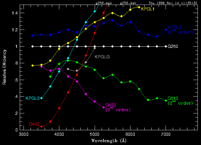
Blue - relative to grating 250
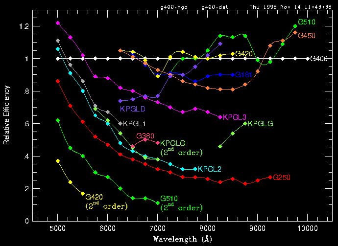
Red - relative to grating 400
Last updated
In addition to other types of calibration data (dome flats, sky flats, milky flats), Hydra uses a system of calibration lamps located in the chimney of the Blanco telescope. This system currently provides the following lamps.
1. Quartz (bright)
2. "Penray" (very bright)
3. Etalon (fairly bright)
4. HeNeAr (dim)
5. Th-Ar (dim)
NOTE: All these lamps (especially He) have finite lifetimes, so please don't leave them turned on unnecessarily for long periods.
The Quartz lamp has no spectral features and can be used for producing flat fields. Unfortunately, the uniformity of the illumination changes with telescope position, making the flats not as useful as dome flats for this purpose, and useless for the fiber-to-fiber throughput measurement needed for good sky subtraction. Where the quartz flats (also known as pflats, for projector flats) are especially useful is providing a trace of the fibers in the field for any given configuration. They are bright and can generally be taken in under a minute of exposure.
This refers to a set of 4 lamps, three of which are Oriel pencil lamps of Ar, Ne and Xe. (Oriel P/Ns 6030, 6032 and 6033). The fourth is a high intensity He lamp, Oriel type #65020. These lamps are very bright and in most cases can give a good calibration exposure in a few seconds. On request, any combination of these lamps can be enabled by Observer Support via switches in the Cass. cage. Individual lamps cannot be selected or deselected from the Hydra console. Thus, if you ask to have only He and Ar turned on, when you select the Penray lamps, it will be an He-Ar source. The relative intensities of the He, Ne and Ar lines which are seen with the Penray lamps are quite diferent from those produced by the HeNeAr lamp because the gasses are at different temperatures, pressures and states of ionization.
This is a collimated quartz lamp illuminating a fused silica Fabry-Perot etalon 0.5mm thick. It produces regularly spaced fringes of high visibility. 3000th order occurs at approximately 4900Å. The fringes are separated by roughly 1.6Å at this wavelength These fringes are quite strong over the spectral range from 5000-8000Å and are useful to some extent above and below these wavelengths. The fringe width is around 1/25 of the separation.
The etalon is potentially very useful for echelle spectroscopy. High resolution reference spectra can be taken rapidly with it and can be calibrated with the penray or Th-Ar lamps. Any drift in the wavelength of the etalon fringes can be quickly detected with a penray exposure. Drift is primarily caused by thermal expansion of the etalon substrate and should be less than 1 ppm/degree C. It is thus unlikely that the wavelengths of the fringes drift by more than 1/20 fringe over the temperature ranges seen on Cerro Tololo.
This is a standard HeNeAr lamp well known to astronomers familiar with the R/C spectrograph. We have a good atlas of the spectral lines produced by this lamp. It is quite dim because of the need to illuminate the entire Hydra field, so it is almost never used.
A standard Th-Ar lamp, identical to the one used in the echelle spectrograph. As in the case of the HeNeAr lamp, the Th-Ar lamp is dim but well understood. An accurate atlas of the lines will be found in the 4M console room. We recommend that observers take long Th-Ar exposures in the afternoon, but rely on the etalon as much as possible for nighttime wavelength calibration.
Click here for an opto-mechanical layout [127] of the calibration lamp system. Light from four of the five calibration lamps is generated in a box located in the Cass. cage of the telescope. A mirror inside this box directs the light from the selected lamp through a liquid-filled light pipe into the chimney where it is projected onto a holographic diffusing screen located on an arm which swings into the beam when the calibration lamps are in use. The penray lamps are located in the chimney and swing automatically into the optical path when used. This location insures that they will be very bright.
A second, larger, spherical mirror swings into the beam at the same time. Light from the diffuser screen is then projected by this spherical mirror onto the Hydra focal plane.
Lamps are selected by buttons on the Hydra GUI [33]. When a lamp button is pressed, the mirrors will move into position and the selected lamp(s) will turn on. When no lamp is selected, the mirrors automatically swing out of the beam. The lamps can also be controlled directly from the TCS operator's console.
Click here for a catalog [128] of available reference spectra and line lists.
|
CTIO HYDRA CALIBRATION LAMP REFERENCE SPECTRA. |
||||
|
Note 1: The 400mm camera has 1.75X the dispersion of the Air Schmidt. Note 2: The direction of the dispersion of raw data is with red at the left. |
||||
| Wavelegth (Å) | Lamp | Grating | Camera | File |
| 3500-6000 | Penray Blue | KPGL1 | Air Schmidt | Plot [129] |
| 3500-6000 | He Blue | KPGL1 | Air Schmidt | Plot [130] |
| 3500-6000 | Ne Blue | KPGL1 | Air Schmidt | Plot [131] |
| 3500-6000 | Ar Blue | KPGL1 | Air Schmidt | Plot [132] |
| 6000-8500 | Penray Red | KPGLF | Air Schmidt | Plot [133] |
| 6000-8500 | He Red | KPGLF | Air Schmidt | Plot [134] |
| 6000-8500 | Ne Red | KPGLF | Air Schmidt | Plot [135] |
| 6000-8500 | Ar Red | KPGLF | Air Schmidt | Plot [136] |
| 5000-5250 | Th-Ar | Echelle (11th order) | 400mm | Plot [137] |
| 5950-6200 | Th-Ar | Echelle (9th order) | 400mm | Plot [138] |
| 6200-6400 | Th-Ar | Echelle (9th order) | 400mm | Plot [139] |
| 6550-6850 | Th-Ar | Echelle (8th order) | 400mm | Plot [140] |
| 6400-6700 | Th-Ar | Echelle (8th order) | Air Schmidt | Plot [141] |
| 6400-6700 | HeNeAr | Echelle (8th order) | Air Schmidt | Plot [142] |
| 7400-8400 | Penray | KPGLD | Air Schmidt | Plot [143] |
| 6400-6700 | Th-Ar | - | - | Line list [144] |
| All | Ne Penray | - | - | Line list [145] |
| All | Ar Penray | - | - | Line list [146] |
| All | He Penray | - | - | Line list [147] |
| All | Hnear | - | - | Line list [148] |
For many years, the fibers used in astronomy have been one of two types - often called "red" and "blue" fibers. Both are made of high quality fused silica with fused silica cladding doped to increase its index of refraction and keep the light contained within the core.
The "red" fibers transmit very well longward of about 500nm, but their internal attenuation rises rapidly in the blue and they are virtually useless below 450nm.
"Blue" fibers are doped with a small amount of OH which greatly improves the transmission at short wavelengths. These fibers are useful well into the UV, the short wavelength limit depending on how long the fibers are. Unfortunately, they have absorption bands in the IR, with a significant reduction in throughput over a narrow band between 700-730nm. Worse attenuation bands appear farther in the IR, beginning at ~850nm, making these fibers almost useless much beyond this wavelength. Transmission curves for fibers of these types are given by fiber manufacturers, such as www.polymicro.com [149]
Internal attenuation in fibers is usually expressed in dB/km. A fiber with an internal attenuation of 10dB/km will reduce the intensity of a beam by half in 333M, while one with 100dB/km attenuation will absorb 50% of the light in 33M. In practical terms, since runs in astronomical fiber-fed spectrographs are seldom more than 30-40M, attenuations of less than 10dB/km are usually negligible, while losses of significantly greater than 100dB/km are unacceptable.
Losses in fiber-fed spectrographs also come from beam spreading or "Focal Ratio Degradation" (FRD for short). All fibers increase the solid angle of slow beams to some extent. The best fibers commercially available can be used in optical systems as slow as f/8. In a high quality, well polished, unstressed modern fiber, 95%+ of the light within an f/8 beam will emerge contained within an f/6-f/7 cone.
In calculating transmissions of fiber-fed spectrographs, one must take into account an additional 7-8% of light loss from reflection at the fiber ends unless the fiber tips can be anti-reflection coated (usually impractical).Even when the fibers are carefully prepared, another 5-15% is generally lost in scattered light produced by polishing imperfections and slight misalignments. In the CTIO Hydra, ~5% of the light is lost at a connector which has been installed in the system to allow Hydra to be removed from the telescope without extracting the fibers.
Thus, even if fiber transmission were perfect, about 75% of the light hitting one end of the CTIO Hydra fibers can be expected to come out the other at an angle at which it can be captured by the spectrograph.
The seeing and accuracy of the fiber positioning further affects the amount of light falling into the fiber. According to Wolffe's standard model for calculating the energy in a seeing disc, 41% of the energy enters a pefectly centered fiber when the fwhm of the seeing disc is equal to the fiber diameter. 68% of the light enters when the seeing disc is 2/3 the diameter of the fiber and 85% will be captured when the seeing disc is half the diameter of the fiber. A comparison of the effect of fibers, slits and and Integral Field Unit (IFU) seeing is shown in this table of efficiencies of aperture types [150]. Sometime during 2000, CTIO Hydra is expected to be equipped with changeable slit masks which will be placed in front of the fibers so that spectral resolution can be maintained even under conditions of less than ideal seeing.
In CTIO Hydra, a new type of fiber has been used, made by Polymicro using a fused slica boule made by Heraus-Amersil. This fiber, sometimes called "STU" fiber combines the best features of red and blue fibers and transmits very well from UV to near IR. This Fiber attenuation graph [151] was measured at CTIO on the Hydra fibers and shows that the attenuation is acceptable at all wavelengths over the spectrograph's design wavelength range from 330-1100nm. The short wavelength limit is determined by the UV cutoff of the glasses used in the ADC corrector. The long wavelength limit is set by the limit of useful sensitivity of silicon CCDs.
The internal transmission in the 36M of fibers in CTIO Hydra is approximately 52% at 340nm, 72% at 400nm, 85% at 500nm and >92% from 600nm-1100nm.
The median seeing on the Blanco telescope is approximately .9 arcsec. CTIO Hydra's positioning is expected to be very good, given astrometric quality coordinates with an rms error of < .2 arcsec.
In practical terms, the large fibers will obviously always collect more light but the spectrograph resolution will be higher and the sky noise will be lower in the small (1.3 arcsec) fibers. Efficiency will be poor under conditions with seeing worse than 2 arcsec, which fortunately constitute a very small fraction of observing time at CTIO.
CTIO Hydra uses fibers 36M long. We can combine all this information to make the following estimate of the overall capture efficiency of the Hydra fibers as a function of seeing and wavelength, assuming perfect centering, 25% loss of light due to end losses and FRD. Attenuation is as measured at CTIO. This table suggests a rule of thumb to use in estimating throughput of Hydra. To first approximation, under average conditions it will be about 1/3 that of a classical spectrograph with a very wide slit.
|
Small (200u) fibers (Not available - reference only) |
|||||
| Seeing | |||||
| Wavelength | .6" | .9" | 1.3" | 1.6" | 2.0" |
| 340nm | .35 | .25 | .16 | .12 | .04 |
| 400nm | .48 | .35 | .22 | .16 | .05 |
| 500nm | .57 | .41 | .26 | .19 | .06 |
| 600-1000nm | .63 | .45 | .28 | .21 | .07 |
|
Large (300u) fibers |
|||||
| Seeing | |||||
| Wavelength | .6" | .9" | 1.3" | 1.6" | 2.0" |
| 340nm | .39 | .35 | .27 | .21 | .16 |
| 400nm | .53 | .49 | .37 | .30 | .22 |
| 500nm | .63 | .57 | .44 | .35 | .26 |
| 600-1000nm | .68 | .62 | .48 | .38 | .28 |
As can be seen from this table, there is no situation in this range of seeing where the small fibers intercept more light than the large fibers. At seeings of .5" or better, the small fibers would gather more light, but images of this quality are rarely, if ever seen at the R/C focus of the Blanco telescope.
In some cases, small fibers would be better because they will intercept less sky or because they will give better resolution in the spectrograph, which was the reason they were installed. However, the small fibers have turned out to be disappointing. They were brittle and a number of them broke on installation. The rest are much less uniform in transmission than the large fibers with only about half of the small fibers having reasonable transmission. They appear to suffer from some kind of manufacturing problem.
Because of their poor quality and limited usefulness, the small fibers have been withdrawn from service and are not currently available. The large fibers work better in virtually all circumstances. Unitl the new 400mm camera / Site 2kx4K CCD combination is available, the resolution attainable with the 300 micron fibers is all that can be reasonably expected. Once the new CCD has been commissioned, observers desiring higher spectral resolution can achieve it by the use of slit plates 200 and 100 microns in width which are available to be inserted in front of the fibers. These will work much better than the present 200 micron fibers under virtually all observing conditions.
t.ingerson
| Aperture Type | Seeing (arcsec) | |||||
| 0.6 | 0.9 | 1.3 | 1.6 | 2.0 | 3.0 | |
| R=50K with 200u Fiber+slit | 0.54 | 0.40 | 0.25 | 0.18 | 0.13 | 0.06 |
| R=50K with 300u Fiber+slit | 0.42 | 0.38 | 0.29 | 0.23 | 0.17 | 0.09 |
| R=50K with Slit only | 0.66 | 0.49 | 0.35 | 0.29 | 0.23 | 0.16 |
| R=50K with 55 fiber IFU | 1.00 | 0.98 | 0.89 | 0.78 | 0.63 | 0.41 |
| R=25K with 200u Fiber (no slit) | 0.89 | 0.65 | 0.41 | 0.30 | 0.21 | 0.10 |
| R=25K with 300u Fiber+slit | 0.77 | 0.70 | 0.54 | 0.43 | 0.32 | 0.17 |
| R=25K with Slit only | 0.93 | 0.79 | 0.62 | 0.53 | 0.44 | 0.30 |
| R=25K with 55 fiber IFU | 1.00 | 0.98 | 0.89 | 0.78 | 0.63 | 0.41 |
| R=16K with 200u Fiber (no slit) | 0.89 | 0.65 | 0.41 | 0.30 | 0.21 | 0.10 |
| R=16K with 300u Fiber (no slit) | 0.99 | 0.90 | 0.69 | 0.55 | 0.41 | 0.22 |
| R=16K with Slit only | 0.99 | 0.93 | 0.81 | 0.71 | 0.61 | 0.44 |
| R=16K with 55 fiber IFU | 1.00 | 0.98 | 0.89 | 0.78 | 0.63 | 0.41 |
ASTRONOMERS ARE NOT ALLOWED TO ENTER THE CASS CAGE WHILE HYDRA IS ON THE TELESCOPE!
Page in Spanish
A continuacion encontraran algunas normas de trabajo y seguridad con HYDRA, espero que con vuestra colaboracion podamos completarlo y/o mejorarlo.
Cuando programa se detiene, por haber tenido dificultades en dejar o tomar alguna fibra,
podriamos intentar lo siguiente en orden de menor a mayor complejidad:
thisis ( o ThisIs 97 )
luego, tratar de mover dicha fibra, por ejm., con commando
park 97.
INSPECCIONAR SOLO VISUALMENTE, SIN INTRODUCIR MANOS NI MENOS LOS BRAZOS, EN REGION AMARILLA, INDICADA EN DIBUJO ADOSADO AL INSTRUMENTO
ADEMAS EL ASISTENTE DE OBSERVACION ES RESPONSABLE DE NO PERMITIR LA COOPERACION DE OTRAS PERSONAS NO ENTRENADAS EN ESTAS LABORES.
Volver a GUI de control, en consola, y tipear
brakes on
en ventana CLI, asegurandose de esta manera que el carro no se desplazara.Terminado de hacer lo propuesto, volver a window CLI y tipear
brakes off.
Si todo funciona en forma normal, volver a posicionar la cortina lateral
brakes on
en instrumento bajar la cortina lateral, desconectar cuatro lockers y, con la presencia de al menos dos personas, bajar la mesa, tratando que no se incline respecto al plano horizontal; al realizar esta operacion, automaticamente, actuan cuatro switches de seguridad posicionados muy cerca de los respectivos cuatro lockers, que tambien desactivan el movimiento del carro.
Si con fibras en problema, no hay otra alternativa de solucion, deben tomarse, con pinzas, para evitar pasar a llevar las cercanas y/o tocarlas con los dedos, y llevarlas, dejandolas apegadas a semicirculo metalico, posicion STOW, anotar el numero de todas las manipuladas. Subir la mesa, reinstalar los seguros, colocar las cortinas laterals; volver a consola y en ventana CLI, tipear
brakes off
y, para cada fibra manipulada, tipear los siguientes dos commandos:
xstowed 105 (indica a programa que esta en posicion stow)
park 105 (la mueve a posicion PARK, a algunos mm de posicion stow, radialmente hacia afuera)
(PRENDER VELITAS A SAN CANTARUTTI, PARA QUE TODO FUNCIONE NORMALMENTE, o, en su defecto un VAYA, VAYA QUE CURIOSO A SAN SCHUMACHER).
quit
pregunta si uno quiere salir de la aplicacion, contestar
yes
pregunta, luego, si uno quiere mover la mesa a la posicion de transporte, contestar
no (a no ser que uno fuera a instalar o retirar el instrumento)
luego pregunta si uno quiere apagar los drives
yes
Al llegar al cage, uno podria, si es extremadamente cauto, en fuente de poder, ubicada a la derecha, apagar, primero, el switch de " Axis drive 115 VAC", y, luego, apagar el de "Logic Supply 115 VAC"
Continuar con los pasos pertinentes de 4a.
NOTA.- Si uno esta ejecutando 4a ,y necesita mover el carro del gripper,debe activar el switch "Safety Override", ubicado en parte interior de caja negra de Galil, ademas de desactivar frenos, en ventana CLI, con
Brakes off
NO OLVIDAR QUE CARRO PUEDE MOVERSE Y CAUSAR DANO. ESTAR MUY ATENTOS AL HABILITARSE EL MOVIMIENTO EN ESTAS CIRCUNSTANCIAS.
Daniel email
Srs:
A Matheson's Oxygen Deficiency Monitor model #8061
was installed inside the Hydra room, the sensor is close to the
refilling area and the unit is in the room next to it (upper right
corner).
It was adjusted at 20.9% as recommended.
A pulsating alarm tone sounds if the oxygen level drops below 19.5%
Effects/Symptoms:
19.5%-21.0% no symptom
14.0%-19.5% Headache, fatigue, faulty judgment
10.0%-14.0% Rise in temperature, difficulty breathing
6.0% -10.0% Convulsions, indistinct consciousness
below 6.0% Coma and heart failure, death in minutes
The unit should be used when work is done in the room,
in special while refilling the dewar.
It uses 2 AA rechargable batteries (steady sound means
battery low). They last ~75 hours, when fully charged.
Sensor's lifetime: 18-24 months, starting today (July 2003).
Accuracy +/- 0.3%
That's all
Danmat S.A
This page collects Hydra engineering reports as they are written. It is intended mainly for use by engineers, Hydra support scientists, and mountain support.
Hydra upgrade plan [152] (Knut Olsen, October 2005)
Hydra cable stretch [153] (Roberto De Propris, March 2009)
Pumping and Dark Current [154] (Roberto De Propris, March 2009)
Status at 2001 Jun 29
Roger Smith
(action items in yellow)
I have invested considerable effort in control of extraneous light sources. Read noise in the SITe 2Kx4K CCD in the Hydra Camera is low enough (3.4 e-) that it can easily be overwhelmed dark current, spurious charge, phosphorescence or light leaks. Recall that
Noise_Floor = SQRT{ read_noise2 + Xbin*Ybin*(Spurious_charge + Dark_Current*time) }
Read Noise (in the overscan) is 3.0 e- for the high gain setting. If the longest exposure time is half an hour, and highest binning factor is 2x2, then we require:
| Spurious_charge | << read_noise2 / (Xbin*Ybin) |
| << 3.02 / (2*2) | |
| << 2 e-/pix |
and,
| Dark_Current | << read_noise2 / (Xbin*Ybin*time) |
| << 3.02 / (2*2*0.5) | |
| << 4.5 e-/pix/hr |
(All figures below are quoted for unbinned pixels.....)
Thus...
| Noise_Floor | = SQRT{ read_noise2 + Xbin*Ybin*(Spurious_charge + Dark_Current*time) } |
| = SQRT{ 3.02 + 2 * 2 *( 0.25 + 0.7 * 0.5 ) } | |
| = 3.4 e- |
2001 August 31
Roger Smith
(action items in green)
Signal to noise in the Hydra Bench Spectrograph is often limited by the noise floor of the detector, which is critically dependent on dark current. Binned by 2 in one or both dimensions, is commonly used to improve the signal to noise ratio or the read time. One must remember that while this helps overcome electronic noise it doesn't help overcome the dark current: binning the signal also bins the dark current.
We have to concern ourselves with all sources of "unwanted signal". Noise in the absence of any astronomical signal is determined by the summation in quadrature of the noise associated with
This is the charge which accumulates per unit time as some electrons in the valence band gain enough energy to overcome the bandgap and jump up into the conduction band. As the detector is cooled the probability that a valence band electron acquires enough energy will drop so that the dark current drops exponentially with temperature. At least this is the case for electrons in a perfect silicon crystal.
In a real device there are imperfections, impurities and crystal dislocations which provide intermediate energy states so that a valence electron can get to the conduction band in two smaller energy steps, increasing the probability of a "thermally generated" conduction band electron. These "hot pixels" produce less dark current with temperature too.
The density of crystal imperfections is greatest at the interface with the oxide layer. Dark current here is suppressed by taking the electrodes negative enough to pull "holes" out of the channel stops (ion implants that create potential barriers between columns). These holes populate the surface of the CCD just under the oxide layer, while the signal charge is repelled to a layer deeper in the CCD. The holes recombine with electrons generated thermally at the surface so that they never reach the storage well.
So, dark current is controlled by lowering the CCD temperature and by maintaining all clock phases negative during integration (MPP mode). The minimum temperature reached by the CCD mount is about 160-165K depending on ambient temperature (radiant load). This should be low enough to ensure good dark current performance. However it was found that dark current always exceeded that expected for the mount temperature measured. The most likely explanation for this is that the CCD is not making good enough thermal contact with the mount and that its temperature is being increased by the radiant load. Fixing this appeared to involve building a new detector mount. Rather than do this the Nitrogen flask is evacuated to promote evaporation/boiling which continues until the remaining liquid solidifies. The temperature drops by 15 degrees in the process and reduces the dark current to an acceptably low level.
Charge injection is the leakage of charge into the image area from the periphery of the CCD during the erase cycle. It can't be erased away since it is smeared across the chip by the erase process. Instead we can clock in reverse at the end of the erase cycle to push it back towards the edge where it originates. I mention it here because it is a serious problem in some of the CCDs in Mosaic which are of the same type, though much less so in this CCD.
Spurious charge is the small amount of charge generated by clocking the CCD. The mechanism is impact ionization: the surface just under the oxide separating the electrodes from the depletion region are populated by holes (due to the negative level on the clocks). This is good since these holes recombine with dark current generated as valence band electrons are excited to conduction band more easily by hopping to the intermediate energy levels produced by interface defects. However as these holes flow back into the channel stops during the rising edges of the clocks they have a low but finite probability of delivering energy to valence electrons which once liberated are collected like signal electrons. At the clock voltages needed to achieve full well, one sees about 2 electrons of spurious charge per pixel implying the probability of generating the spurious electron is about 1 in 2000 per shift.
When high gain is sleeted in the setdetector menu, the waveform compiler embeds commands in the new waveform macro which reduces the high levels of the parallel clocks. This reduces the spurious charge to an acceptable level at the expense of full well. When the high gain setting is selected the well capacity is reduced to 15000 e-. At 0.84e-/ADU this represents 18000 ADU, but when binned 2x2 exceeds the ADC range by about 10% so the loss in well capacity will often not be noticed.
Obviously light leaking into the spectrograph masquerades as dark current and has exactly the same effect. While light leaks are in principal very simple to understand there is an extensive set of tips in the section on Eliminating Light Leaks, which you should read if you detect a problem.
Check for light leaks (etc) before each observing block !....
It is most likely that to maintain full sensitivity of the spectrograph it will be necessary to verify that all of these "dark signals" are within normal bounds prior to each observing block. To do this take the following full frame exposures with binning set to 2x2.
If the dark signal is abnormally high, even when dome and surrounding room lights are off, check that no abnormal or unauthorized objects have been left in the room which may be phosphorescing. For example the paint on some nitrogen dewars may glow in the dark, too faintly to see by eye but enough to affect the CCD. Unless you find a simple explanation like this, don't waste time guessing about the cause: you should use a cooled CCD and camera lens to image the bench spectrograph room.
Recall that
| Noise_Floor = |
SQRT{ read_noise2 + Xbin*Ybin*(Spurious_charge + [Dark_Current + light_leak]*time) } |
Read Noise (in the overscan) is 3.0 e- for the high gain setting. Assuming that the highest binning factor is 2x2, then we require:
| Spurious_charge | << read_noise2 / (Xbin*Ybin) |
| << 3.02 / (2*2) | |
| << 2 e-/unbinned_pixel |
and if the longest exposure time is half and hour, then we require:
|
Dark_Current + Light_leaks |
<< read_noise2 / (Xbin*Ybin*time) |
| << 3.02 / (2*2*0.5) | |
| << 4.5 e-/unbinned_pixel/hour |
When all is working correctly,
| Noise_Floor | = SQRT{ read_noise2 + Xbin*Ybin*(Spurious_charge + Dark_Current*time) } |
| = SQRT{ 3.02 + 2 * 2 *( 0.25 + 0.7 * 0.5 ) } | |
| = 3.4 e- |
This has not been as simple as one might think! Here are some tips....
Many materials absorb light then re-emit it over a long period of time. This can cause a dark current which decays over time and is thus harder to pin down. It is therefore important to not leave any item inside the room unless it is essential and has been proven to be free from phosphorescence. These are some examples which have been addressed:
If no obvious source is found after consulting the above checklists, don't waste time guessing. Use a cooled CCD camera fitted with a camera lens and integrating for 2-5 minutes to identify light sources. The following setup is very effective:
Sometimes it can be difficult to figure out exactly what you are looking at in the noisy dark images. In this case it helps to take a short exposure without moving the camera leaving a low light source on in the room. Use the smallest aperture and low light such as leaving the door open into the anteroom. Be careful not to be confused by reflections from the metallic surfaces or by the light emitted by the arcon you are using. Its data fibers need to be taped over and it needs to be wrapped in black cloth. To avoid spending all day in the elevator, get an assistant at the keyboard downstairs or setup a laptop on the network to provide a local terminal for controlling Arcon.
The following notes were made during commissioning
and are left here for completeness
though some of the information is duplicated.
November 2001
Knut Olsen, on behalf of the people who work on Hydra: Rolando Cantarutti, Rodolfo Cardemil, Manuel Martinez, Daniel Maturana, Andres Montane, Javier Rojas, Oscar Saa, Nick Suntzeff, Ricardo Venegas
The Hydra spectrograph and positioner have had a history of problems since its commissioning. In the months July-September 2001, good progress was made towards fixing the worst problems. Below are summaries of the problems we have encountered and the work done to fix them.
The problems with the positioner resulted in the loss of often several hours per night.
Many thanks to Sam Barden, Phil Massey, Dave Sawyer, and Bezhad Aredeshi for their advice on fixing Hydra's troubles.
Our top priority for Hydra before the October 2001 observing block was to reduce the failure rate of the gripper. Many of the problems experienced in previous runs, listed above, have now been fixed:
However, with the appearance of another problem with the gripper (#3), it became clear that a complete overhaul of the gripper was necessary. Andres Montane (hardware) and Rolando Cantarruti (software) jointly took on this work, with Ricardo Venegas supporting.
 [155]
[155]
Fig. 1. Close-up of gripper assembly
In order to uncover the cause of the gripper troubles, Andres & Co. needed to understand how the gripper behaves during the sequence of picking up a button, moving it, and putting it back onto the plate. What is supposed to happen? From Sam Barden:
The gripper thus cycles through three states while placing a button: open, closed, and relaxed. (A fourth state, "open wide", is also available, but is used mainly when the gripper is initialized). How does the gripper achieve these states? In Fig. 1 above, the three teeth of the gripper are mounted on the black wheel with red LEDs attached. When this wheel rotates, the teeth tilt about their mounting pins and the jaw opens or closes. The motor which provides the power to rotate the wheel is located immediately above the label "C". "A"-"D" indicate four mechanical switches. From our observations of the gripper in April 2001 and conversation with Sam Barden, we established that:
Andres&Co. independently established these functions of the switches. Their real insight, however, came from Andres' understanding of the mechanics of the system. Andres first observed that the turning of the gripper motor compresses the spring in switch C and opens the gripper. The closing of the gripper is then entirely driven by the stored tension in the spring. Second, given the distance by which the teeth are supposed to move in order to reach the open position, Andres calculated the distance through which the motor needs to turn. He found that the motor was stopping before it reached the full open position, held back by excessive force from the spring and by a spring in switch B. After he adjusted the positions of switches B and C, the gripper was able to complete the opening of the jaws. (Incidentally, Rolando discovered that the setting of switch B is never used in the software control, so that it actually serves no purpose). Third, Andres noted that when closing the gripper with a button in the jaw, the teeth continued to rotate even after they were fully closed around the gripper. By tuning switch A, he was able to stop the closing of the jaw before the teeth imparted rotation to the button.
Following Andres', Rolando's, and Ricardo's work on the gripper, the October observing block passed with no trips to the cage to untangle problems with the fibers, and virtually zero problems with the gripper. Their work leaves us with two valuable lessons:
Andes will refine the process of tuning the gripper before the next Hydra block.
 [156]
[156]
Fig. 2. Heads of arrows are current FOPS fiber positions, tails are positions before commissioning
Page in Spanish
Detector, dewar and Arcon work, Ramon Galvez H., June 2002
More detector, dewar and Arcon work - Ramon Galvez , August 16th, 2002
| CCD dwr vac before pumping | : 300 Torr |
| CCD dwr vac after pumping | : 0 mT |
| LN2 flask vac after refill | : 400 Torr |
| LN2 flask vac for solid state | : 20 Torr ( after 1hr pumping ) |
Ramon will check out the vacuum and prepare a new molecular sieve during the week of 21/3
On the next engineering night, we will measure the rotation near the equator and adjust x_offset and y_offset by going to the pole.
Rolando is looking at exactly how big the axial alignment error is.
Can Roberto check the optical alignment soon?
Rolando will add a fix to the code
First, Hernan, Ricardo, Knut, Daniel, and Patricio will write up a detailed set of procedures, hints, and tricks for doing the echelle setup
We want to investigate getting replacement ThAr lamps--Oscar will contact Kitt Peak to find out what they are using
Observer support will check out what is currently in the chimney.
Oscar and Knut will contact Kitt Peak about what lamps they have and who supplies them
Hernan, Oscar, Ricardo, Knut, Patricio will also make a web page listing all of our comparison lamp supplies
Andres and Ricardo will check out the z-limit switch and the general mechanical tuning of the gripper during the week of 21/3. Andres will also see whether a new z-limit switch design may be implemented before April 16, 2004.
The trouble with the erratic limit switch signals was solved by replacing the spare Galil with the original Galil. Trouble is that the original Galil had some problems of its own, such as getting lost and producing "x-y stage not at destination" errors. The Galil boxes have been sent back to the company twice for repair, but have been returned with the statement that there is nothing wrong with them. Gale will ask Galil for a quote on a new replacement.
FIXED after David changed the values and Rolando incorporated the fix into automated software.
Given that generally our hydraassign files successfully positioned fibers further from the pole, and without any problems at the WIYN fiber instrument in more than three hundred pointings over the last four years our experience suggests that possibly the positioning troubles find their explanation in a residual telescope polar alignment error. Mr. Bremer had remarked that the Blanco Telescope has a significant residual alignment error, as do many if not all equatorially mounted telescopes.
While Wallace's pointing model and correction software does reduce telescope pointing discrepancies, canceling the error on-axis, we wonder if the field rotation correction coefficients that Wallace\'s software produces are passed to the hydra software. Were they not read by hydra, then a three arc-minute telescope misalignment could produce major problem when hydra attempts to observe near the pole.
We would be grateful if this possibility could be looked into, possibly allowing for manual keyboard entry (or its equivalent) of the pointing model generated coefficients. In particular, we should be grateful if this might be resolved on the April 16th engineering night, so that our next observer working on this project April 17th through the 19th could do the fields we had to delete from our current observing program that was, in other respects, highly successful.
Hydra Status Report, Notes from the meeting April 2000 - Updates 2002, 2003
Knut Olsen, 4/3/2002
Updated 5/24/2002
Updated 7/14/2003
People and jobs assigned, in order of priority. See list below for job descriptions. Updates in light blue.
Srs:
A Matheson's Oxygen Deficiency Monitor model #8061 was installed inside the Hydra room, the sensor is close to the refilling area and the unit is in the room next to it (upper right corner). It was adjusted at 20.9% as recommended. A pulsating alarm tone sounds if the oxygen level drops below 19.5%
Effects/Symptoms:
19.5%-21.0% no symptom
14.0%-19.5% Headache, fatigue, faulty judgment
10.0%-14.0% Rise in temperature, difficulty breathing
6.0% -10.0% Convulsions, indistinct consciousness
below 6.0% Coma and heart failure, death in minutes
The unit should be used when work is done in the room, in special while refilling the dewar.
It uses 2 AA rechargable batteries (steady sound means battery low). They last ~75 hours, when fully charged.
Sensor's lifetime: 18-24 months, starting today (July 2003). Accuracy +/- 0.3%
That's all
Danmat S.A
Buenas Noticias,
Thank Manuel Martinez and Unisite (the ETS device programmer) the brand new flash eprom and the bad one from the spare galil could be programmed. The eprom in the original Galil (the only good one we had) served as master and Manuel made a backup of its content. The original Galil and the spare Galil are functioning now. I let run a largecircle and a parklarge with each eprom. No one error happened. It seems that our Galil units aren't able to program the flash eproms or I'm unable to get them burnt. I got the programs into the eproms but the burn in command produced a timeout error only.
We still have two virgin eproms. I'll send them to Manuel for programming. I think, it isn't worth to investigate, why our galil doesn't program the eproms, because the Unisite can do it better. It looks like the trouble with the hydra spares will be then over for the next time.
Saludos
Javier
Here is a quick summary of the topics discussed at the Hydra meeting on August 23, 2004, and the conclusions we reached:
There are two basic solutions. One is to buy a motor and external encoder and use the existing, now-defunct SMC connection for the shutter operation to operate the motor. May be a significant mechanical design effort, however. The second is to replace the existing manual micrometer with a motorized version. This is mechanically easy, but communication with the SMC requires study.
--> Andres, Manuel, Enrique, Javier, Ricardo, Rodolfo will study the problem
Need to ensure that the pellicle may be replaced without damage.
--> Ricardo and Andres will discuss
Several apparent z-limit switch failures even after redesign and installation by Andres.
--> Javier and Enrique will try to reproduce the problem on the next turno, and write a proposal for a solution
--> send Knut any items you can think of
The first three refer to the z-axis failures referred to above.
The next two refer to failure of the guider, the solution of which was reported in #502. But we need either spare VME cards, or perhaps Rolando's software patch.
--> Enrique and Javier wil discuss with Rolando
The last (320) refers to the broken echelle filter #6.
--> Knut will discuss finding a replacement with Roberto
Exists, but doesn't work. Why?
--> Knut will look into it.
By Charles Corson, February 2010.
There are a great number of things that can cause the linear actuator to fail. I would first decouple it from the linear actuator from the articulation arm, the straight piece which comes down from the gripper face.
This decoupling is very simple: you remove the jam nut on the end of the ball screw at the left end of the actuator. Once done, you command the gripper to open and close.
What you are looking for is a smooth, consistent in/out motion of the balls screw, the linear actuation. Without any mechanical loading, this should be a simple test of the actuator itself. If it appears to be 'sticking', you can apply a drop or two of light lubricant. I've seen these actuators fail because the original lubricant has 'gummed' up, become dry and very sticky, waxy. You also want to look closely at the linear keyway on the ball screw. You will see just at that face of the teflon nut, a teflon key, or tab, that fits directly into that slot. The Tab should be in good shape, not rounded, or deformed. If it is, the ball screw is likely turning with the motor under high load and then there is a complete loss of linear actuation. The ball screw must have no rotation in relation to the motor turns. Of course, it rotates within the nut.
Let us assume that the linear actuator is good with no mechanical load. I would then be highly suspect of the various mechanical adjustments: position of jam nut for correct 'relax' tension on the button, position of the close 'stop', position of the 'open' stop. There is no easy way to explain this fully, adequately. I've found that it is an iterative tuning so that OPEN is at the correct position, N-steps produces the correct relative position for 'relax' state, and the right position for close. To throw one more adjustment in the mix, one then has to have the 'tension' the spring force of the jam nut and spring on the linear actuator at the right state.
Here is YET ANOTHER issue to consider. There is a IC stepper driver on the controller card. Under mechanical load, if this driver is 'bad' or over-heating, the stepper will stall of course.
Don't assume all gripper failures have to do with the motor.
(last updated February 2012)
If we have missed one of your Hydra-CTIO publications, please email instrument scientist David James at djames ctio noao edu
| Input Parameters | Derived Information | ||||||
| Wavelength: | 4250Å | Grating Angle | 7.72° | Slit Transmission | 1 | ||
| Grating: | KPGL1 | Lines/mm | 632 | Blaze | 4200Å | ||
| Order: | 1 | Best Wavelength | 4200Å | Grating Efficiency | 0.80 | ||
| Slit Plate: | None | Dispersion | 39.2Å/mm | Resolution: | 1205 | ||
| Filter: | None | Scale | 0.59Å/pixel | Coverage: | 2408Å | ||
| Camera: | SITE400mm | Camera Focal Length | 400 mm | Incident photons/sec | 15.21/resel | ||
| Seeing: | 1" | Seeing disc in fiber | 0.87 | Detected photons/sec | 0.51/resel | ||
| Air Mass: | 1.2 | Atmosphere Trans. | 0.74 | Sky photons/sec | 0.65 | ||
| Binning: | 1 | Fiber transmission | 0.81 | Detected sky photons/sec | 0.02 | ||
| Moon: | 7 | Filter transmission | 1.00 | System Efficiency | 0.034 | ||
| Target Mag.: | 17 | S/N ratio: | 30 | Exposure Time* | 2078 sec. |
*In a fiber-fed spectrum there
is no spatial information in the direction perpendicular to the
dispersion. In principle one could bin the CCD in this direction to
reduce readout noise. In practice this is seldom possible because of
camera distortion. One usually reads the entire CCD and extracts a
1-D spectrum in software. Such a spectrum has a noise in each
resolution element (resel) equivalent to that produced by a number of
CCD reads equal to the projected width of the fiber on the CCD. The
calculated exposure time is that predicted to yield an extracted 1-D
spectrum with the specified S/N in each resel.
Last updated 3 May 2006 - Knut Olsen
Links
[1] ftp://ftp.ctio.noao.edu/ctio/hydra/hydrasimSolaris.tar.Z
[2] ftp://ftp.ctio.noao.edu/ctio/hydra/hydrasimLinux.tar.gz
[3] http://www.ctio.noao.edu/noao/sites/default/files/instruments/spectrographs/concentricitieslarge.txt
[4] http://www.ctio.noao.edu/noao/sites/default/files/instruments/spectrographs/alternating_concentricities
[5] http://www.ctio.noao.edu/noao/sites/default/files/instruments/spectrographs/hydraslitids.txt
[6] http://www.ctio.noao.edu/noao/content/hydra-safety
[7] http://www.ctio.noao.edu/noao/content/focus-throughput
[8] http://www.ctio.noao.edu/noao/content/temperature-focus-relationship-hydra
[9] http://www.ctio.noao.edu/noao/content/ctio-hydra-users-manual#lost-fibers
[10] http://www.ctio.noao.edu/noao/content/ctio-hydra-users-manual#collisions
[11] http://www.ctio.noao.edu/noao/content/rcadc-and-atmospheric-refraction
[12] http://www.ctio.noao.edu/noao/content/smc-commands#a
[13] http://www.ctio.noao.edu/noao/content/smc-commands#b
[14] http://www.ctio.noao.edu/noao/content/how-use-tv-camera-chimney
[15] http://www.ctio.noao.edu/noao/content/fops-alignment
[16] http://www.ctio.noao.edu/noao/sites/default/files/instruments/spectrographs/hydrawiynmanual.ps
[17] http://www.ctio.noao.edu/noao/sites/default/files/instruments/spectrographs/periscope.gif
[18] http://www.ctio.noao.edu/noao/content/software-0
[19] http://www.ctio.noao.edu/~olsen/IDL/hydrapro.tar
[20] http://www.ctio.noao.edu/noao/content/mosaic-ii-ccd-imager
[21] http://iraf.noao.edu/projects/ccdmosaic/astrometry/astrom.html
[22] http://vizier.u-strasbg.fr/cgi-bin/VizieR
[23] http://www.ctio.noao.edu/noao/content/init-status-script-and-coord-files
[24] http://www.ctio.noao.edu/noao/content/Software-0
[25] http://www.ctio.noao.edu/noao/content/Knuts-Hydra-Notes
[26] http://archive.eso.org/skycat/servers/ASTROM
[27] http://www.astro.yale.edu/dokkum/lacosmic/
[28] http://www.ctio.noao.edu/noao/sites/default/files/instruments/spectrographs/finalslit
[29] http://www.ctio.noao.edu/noao/sites/default/files/Facilities/Documents/97_VNC.pdf
[30] mailto:hydra@ctiozm
[31] http://www.ctio.noao.edu/noao/content/How-obtain-Hydra-CTIO-Simulator
[32] ftp://ftp.noao.edu/ctio
[33] http://www.ctio.noao.edu/noao/sites/default/files/instruments/spectrographs/hydra_gui.gif
[34] http://www.ctio.noao.edu/noao/content/tcs-commands
[35] http://www.ctio.noao.edu/noao/content/tcs-router
[36] http://www.ctio.noao.edu/noao/content/Embedded-Galil-Software-Coding-Standard
[37] http://www.ctio.noao.edu/noao/sites/default/files/instruments/spectrographs/hydraassign.ps
[38] ftp://ftp.ctio.noao.edu/ctio/hydra/lepusastrom.hydra
[39] http://www.ctio.noao.edu/noao/content/measuring-concentricities
[40] http://www.ctio.noao.edu/noao/content/user-interfase#execfile
[41] http://www.ctio.noao.edu/noao/content/user-interfase#configure
[42] http://www.ctio.noao.edu/noao/content/hydraassign
[43] http://www.ctio.noao.edu/noao/content/hydra-cli-coldstar
[44] http://www.ctio.noao.edu/noao/content/hydra-cli-home
[45] http://www.ctio.noao.edu/noao/content/hydra-cli-minit
[46] http://www.ctio.noao.edu/noao/content/hydra-cli-brakes
[47] http://www.ctio.noao.edu/noao/content/hydra-cli-gox
[48] http://www.ctio.noao.edu/noao/content/hydra-cli-goy
[49] http://www.ctio.noao.edu/noao/content/hydra-cli-goxy
[50] http://www.ctio.noao.edu/noao/content/hydra-cli-gotag
[51] http://www.ctio.noao.edu/noao/content/hydra-cli-goz
[52] http://www.ctio.noao.edu/noao/content/hydra-cli-gripin
[53] http://www.ctio.noao.edu/noao/content/hydra-cli-gripout
[54] http://www.ctio.noao.edu/noao/content/hydra-cli-tag
[55] http://www.ctio.noao.edu/noao/content/hydra-cli-view
[56] http://www.ctio.noao.edu/noao/content/hydra-cli-gopen
[57] http://www.ctio.noao.edu/noao/content/hydra-cli-relax
[58] http://www.ctio.noao.edu/noao/content/hydra-cli-gclose
[59] http://www.ctio.noao.edu/noao/content/hydra-cli-openwide
[60] http://www.ctio.noao.edu/noao/content/hydra-cli-griptest
[61] http://www.ctio.noao.edu/noao/content/hydra-cli-abump
[62] http://www.ctio.noao.edu/noao/content/hydra-cli-bump
[63] http://www.ctio.noao.edu/noao/content/hydra-cli-offset
[64] http://www.ctio.noao.edu/noao/content/hydra-cli-dropit
[65] http://www.ctio.noao.edu/noao/content/hydra-cli-mark
[66] http://www.ctio.noao.edu/noao/content/hydra-cli-move
[67] http://www.ctio.noao.edu/noao/content/hydra-cli-park
[68] http://www.ctio.noao.edu/noao/content/hydra-cli-thisis
[69] http://www.ctio.noao.edu/noao/content/hydra-cli-thisis-0
[70] http://www.ctio.noao.edu/noao/content/hydra-cli-unstow
[71] http://www.ctio.noao.edu/noao/content/hydra-cli-aload
[72] http://www.ctio.noao.edu/noao/content/hydra-cli-assign
[73] http://www.ctio.noao.edu/noao/content/hydra-cli-configure
[74] http://www.ctio.noao.edu/noao/content/hydra-cli-config1
[75] http://www.ctio.noao.edu/noao/content/hydra-cli-preview
[76] http://www.ctio.noao.edu/noao/content/hydra-cli-save
[77] http://www.ctio.noao.edu/noao/content/hydra-cli-setup
[78] http://www.ctio.noao.edu/noao/content/hydra-cli-setup-field-command
[79] http://www.ctio.noao.edu/noao/content/hydra-cli-configmode
[80] http://www.ctio.noao.edu/noao/content/hydra-cli-concenmode
[81] http://www.ctio.noao.edu/noao/content/hydra-cli-flexmode
[82] http://www.ctio.noao.edu/noao/content/hydra-cli-thermmode
[83] http://www.ctio.noao.edu/noao/content/hydra-cli-scalemode
[84] http://www.ctio.noao.edu/noao/content/hydra-cli-lit
[85] http://www.ctio.noao.edu/noao/content/hydra-cli-ping
[86] http://www.ctio.noao.edu/noao/content/hydra-cli-dangle
[87] http://www.ctio.noao.edu/noao/content/hydra-cli-hangle
[88] http://www.ctio.noao.edu/noao/content/hydra-cli-setcable
[89] http://www.ctio.noao.edu/noao/content/hydra-cli-thermval
[90] http://www.ctio.noao.edu/noao/content/hydra-cli-hist
[91] http://www.ctio.noao.edu/noao/content/hydra-cli-listdump
[92] http://www.ctio.noao.edu/noao/content/hydra-cli-listtag
[93] http://www.ctio.noao.edu/noao/content/hydra-cli-status
[94] http://www.ctio.noao.edu/noao/content/hydra-cli-where
[95] http://www.ctio.noao.edu/noao/content/hydra-cli-whereis
[96] http://www.ctio.noao.edu/noao/content/hydra-cli-purge
[97] http://www.ctio.noao.edu/noao/content/hydra-cli-restore
[98] http://www.ctio.noao.edu/noao/content/hydra-cli-xparked
[99] http://www.ctio.noao.edu/noao/content/hydra-cli-xstowed
[100] http://www.ctio.noao.edu/noao/content/hydra-cli-zdb
[101] http://www.ctio.noao.edu/noao/content/hydra-cli-listti
[102] http://www.ctio.noao.edu/noao/content/hydra-cli-listts
[103] http://www.ctio.noao.edu/noao/content/hydra-cli-inputchart
[104] http://www.ctio.noao.edu/noao/content/hydra-cli-swchart
[105] http://www.ctio.noao.edu/noao/content/hydra-cli-execfile
[106] http://www.ctio.noao.edu/noao/content/hydra-cli-complamp
[107] http://www.ctio.noao.edu/noao/content/hydra-cli-plate
[108] http://www.ctio.noao.edu/noao/content/hydra-cli-quit
[109] http://www.ctio.noao.edu/noao/content/how-obtain-hydra-ctio-simulator
[110] http://www.ctio.noao.edu/noao/content/user-interfase#listdump
[111] http://www.ctio.noao.edu/noao/content/hydra-cli-coldstart
[112] http://www.ctio.noao.edu/noao/content/init-status-script-and-coord-files#concentricities
[113] http://www.ctio.noao.edu/noao/content/init-status-script-and-coord-files#astroparams
[114] http://www.ctio.noao.edu/noao/content/init-status-script-and-coord-files#systemparams
[115] http://www.ctio.noao.edu/noao/content/embedded-galil-software-files
[116] ftp://ftp.noao.edu/ctio/hydra
[117] http://www.ctio.noao.edu/noao/content/SMC-Commands
[118] http://www.ctio.noao.edu/noao/content/HBS-400-mm
[119] http://www.ctio.noao.edu/noao/content/HBS-229mm
[120] http://www.ctio.noao.edu/noao/sites/default/files/instruments/spectrographs/HBS_400mm.gif
[121] http://www.ctio.noao.edu/noao/content/hydra-spectrograph-gui#3
[122] http://www.ctio.noao.edu/noao/content/Gratings-Hydra-Multiple-Object-Spectrograph
[123] http://www.ctio.noao.edu/noao/sites/default/files/instruments/spectrographs/HBS_229mm.gif
[124] http://www.ctio.noao.edu/noao/content/gratings-hydra-multiple-object-spectrograph
[125] http://www.ctio.noao.edu/noao/content/calibraction-lamps
[126] http://www.ctio.noao.edu/noao/content/echelle-mode
[127] http://www.ctio.noao.edu/noao/sites/default/files/instruments/spectrographs/chimney_layout.gif
[128] http://www.ctio.noao.edu/noao/content/reference-spectra
[129] http://www.ctio.noao.edu/noao/sites/default/files/instruments/spectrographs/Penrayblue.gif
[130] http://www.ctio.noao.edu/noao/sites/default/files/instruments/spectrographs/heblue.gif
[131] http://www.ctio.noao.edu/noao/sites/default/files/instruments/spectrographs/neblue.gif
[132] http://www.ctio.noao.edu/noao/sites/default/files/instruments/spectrographs/arblue.gif
[133] http://www.ctio.noao.edu/noao/sites/default/files/instruments/spectrographs/penrayred.gif
[134] http://www.ctio.noao.edu/noao/sites/default/files/instruments/spectrographs/hered.gif
[135] http://www.ctio.noao.edu/noao/sites/default/files/instruments/spectrographs/nered.gif
[136] http://www.ctio.noao.edu/noao/sites/default/files/instruments/spectrographs/arred.gif
[137] http://www.ctio.noao.edu/noao/sites/default/files/instruments/spectrographs/5186.gif
[138] http://www.ctio.noao.edu/noao/sites/default/files/instruments/spectrographs/6027.gif
[139] http://www.ctio.noao.edu/noao/sites/default/files/instruments/spectrographs/6371.gif
[140] http://www.ctio.noao.edu/noao/sites/default/files/instruments/spectrographs/6757.gif
[141] http://www.ctio.noao.edu/noao/sites/default/files/instruments/spectrographs/thar1.gif
[142] http://www.ctio.noao.edu/noao/sites/default/files/instruments/spectrographs/henear2.gif
[143] http://www.ctio.noao.edu/noao/sites/default/files/instruments/spectrographs/penray74_84.gif
[144] http://www.ctio.noao.edu/noao/sites/default/files/instruments/spectrographs/thar64-67.dat
[145] http://www.ctio.noao.edu/noao/sites/default/files/instruments/spectrographs/hydne.dat
[146] http://www.ctio.noao.edu/noao/sites/default/files/instruments/spectrographs/hydar.dat
[147] http://www.ctio.noao.edu/noao/sites/default/files/instruments/spectrographs/hydhe.dat
[148] http://www.ctio.noao.edu/noao/sites/default/files/instruments/spectrographs/hydhenear.dat
[149] http://www.polymicro.com/
[150] http://www.ctio.noao.edu/noao/content/efficiency-aperture-types
[151] http://www.ctio.noao.edu/noao/sites/default/files/instruments/spectrographs/CTIO_fiber_atten.gif
[152] http://www.ctio.noao.edu/noao/sites/default/files/instruments/spectrographs/UpgradePlan.doc.pdf
[153] http://www.ctio.noao.edu/noao/sites/default/files/instruments/spectrographs/Fibers.pdf
[154] http://www.ctio.noao.edu/noao/sites/default/files/instruments/spectrographs/hydra_dc.pdf
[155] http://www.ctio.noao.edu/noao/sites/default/files/instruments/spectrographs/gripperlab.jpg
[156] http://www.ctio.noao.edu/noao/sites/default/files/instruments/spectrographs/fops2.gif
[157] http://www.ctio.noao.edu/noao/content/Hydra-Dark-Current-II-Keeping-dark-current-low-2001
[158] http://www.ctio.noao.edu/noao/content/peter-frinchaboy-bill-kunkels-mail
[159] http://www.ctio.noao.edu/noao/content/daniels-email
[160] http://www.ctio.noao.edu/noao/content/maintenance-work-between-observing-blocks
[161] http://www.ctio.noao.edu/noao/content/javiers-email
[162] http://adsabs.harvard.edu/abs/2012ApJ...749..175J
[163] http://adsabs.harvard.edu/abs/2011ApJ...732..108J
[164] http://adsabs.harvard.edu/abs/2011AJ....141...58J
[165] http://adsabs.harvard.edu/abs/2010AJ....139.1871W
[166] http://adsabs.harvard.edu/abs/2010ApJ...722.1373J
[167] http://adsabs.harvard.edu/abs/2009ApJ...703..894H
[168] http://adsabs.harvard.edu/abs/2009ApJ...702L.153H
[169] http://adsabs.harvard.edu/abs/2009ApJ...698.2048J
[170] http://adsabs.harvard.edu/abs/2008ApJ...688.1060H
[171] http://adsabs.harvard.edu/abs/2008AJ....136..118F
[172] http://adsabs.harvard.edu/abs/2008ApJ...681.1505J
[173] http://adsabs.harvard.edu/abs/2007ApJ...658L..29R
[174] http://adsabs.harvard.edu/abs/2006ApJ...648..580H
[175] http://adsabs.harvard.edu/abs/2005AJ....130.2677M
[176] http://adsabs.harvard.edu/abs/2004AJ....127.2674O
[177] http://adsabs.harvard.edu/abs/2004AJ....127.3411C
[178] http://adsabs.harvard.edu/abs/2003AJ....126..762C