Calibration Data

Calibration Data for Mosaic Reductions

16 Channel Mode:

CCD test data for 16 channel mode [1]

Photometric zero terms for 16 channel mode [2] and sky rates [3].

Bad pixel masks for 16 channel mode [4]

WCS, Crosstalk and CCD data for 16 channel mode [5] courtesy Armin Rest and the SMSN collaboration (March 2008)

8 Channel Mode:

CCD test data for 8 channel mode [6].

Crosstalk file for 8-channel mode [7]

WCS file for 8-channel mode, [8] courtesy Eduardo Balbinot (March 2010)

Bad Pixel Mask for 8-channel mode [9], with help from Frank Winkler and Knox Long (May 2010)

* Previous calibrations and information on Mosaic II [10].

CCD test data for 16 channel mode

Report, 2002-05-17 [11] (brief)

Full frame, unbinned, dual redout:

CCD (1)	1a	1b	2a	2b	3a	3b	4a	4b
FITS section	1	2	3	4	5	6	7	8
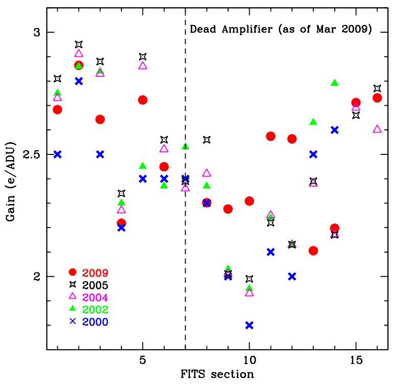
Gain (e-/ADU) 09 Nov 2009 (2)	2.7	2.8	2.7	2.3	2.8	2.5	N/A	2.3

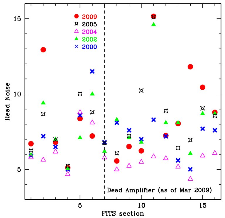
Read noise (e-) 09 Nov 2009 (3)	6.7	12.8	7.0	5.2	8.4	7.2	N/A	5.6

Non- linearities 17 May 2002 (4)	~<1%	~<1%	~<1%	~<1%	~<1%	~<1%	~<0.8%	~<1%
Non- linearities Oct 2005 (4)	~<1%	~<1%	~<1%	~<1%	~<1%	~<1%	~<1%	~<1%

Spurious charge (ADU) 17 May 2002 (5)	N/M	~10	~5	~8	~10	~12	~15	~8

Full well (e-) 08 May 2004 (6)	130,000	125,000	91,000	87,000	77,000	81,000	70,000	71,000
Full well (e-) Oct 2005 (7)	>112,000	>118,000	86,000	89,000	87,000	97,000	67,000	67,000

CCD (1)	5b	5a	6b	6a	7b	7a	8b	8a
FITS section	9	10	11	12	13	14	15	16
Gain (e-/ADU) 09 Nov 2009 (2)	2.3	2.3	2.6	2.6	2.1	2.2	2.7	2.7

Read noise (e-) 09 Nov 2009 (3)	6.4	6.2	15.2	7.3	7.9	12.0	10.4	8.7

Non- linearities 17 May 2002 (4)	~<1%	~<1%	~<1%	~<1%	~<1%	~<1%	~<1%	~<1%
Non- linearities Oct 2005 (4)	~<1%	~<1%	~<1%	~<1%	~<1%	~<1%	~<1%	~<1%

Spurious charge (ADU) 17 May 2002 (5)	~-5	~-5	~-5	~-5	~-2	~-2	~-5	~-5

Full well (e-) 08 May 2004 (6)	76,300	84,000	97,000	102,000	95,500	93,000	62,000	67,600
Full well (e-) Oct 2005 (7)	76,000	80,000	73,000	81,000	91,500	100,000	56,000	61,000

Notes:

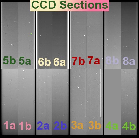
1. When looking at a Mosaic image, the 8 lower segments are denoted from left to right (ccd,amp) 1a,1b,2a,2b,3a,3b,4a,4b. Across the top, from left to right: 5b,5a,6b,6a,7b,7a,8b,8a (see plot below).

2. Gain measured from Transfer curve.

3. Read noise calculated from standard deviation of a bias frame × gain.

4. Nonlinearities are the width of the envelope of the count rate curve over a large part of the dynamic range of the detector. They include any variation in the light source and shutter effects, although the shutter delay has been removed to first order. These measurements are therefore an upper bound.

5. Spurious charge is charge that is injected into the CCD as a result of parallel clocking. It shows up as a slope in the bias level in the vertical direction, quoted here in ADUs from the top to the bottom of the unbinned image.

6. Measured in the La Serena lab after the installation of a new CCD #3. Full well was determined from the variance curve, noise from the overscan.

7. Measured in situ at Blanco prime focus, using flat field lights.

Photometric Zero Points & Color Terms

Last updated: K. Olsen 27 August 2003

		Chip 1	Chip 2	Chip 3	Chip 4	Chip 5	Chip 6	Chip 7	Chip 8
Zero Point	U	2.217 (0.007)	2.220 (0.005)	2.231 (0.005)	2.254 (0.008)	2.234 (0.010)	2.215 (0.005)	2.216 (0.005)	2.227 (0.009)
	B	-0.107 (0.008)	-0.120 (0.008)	-0.115 (0.008)	-0.111 (0.009)	-0.111 (0.008)	-0.101 (0.008)	-0.106 (0.008)	-0.104 (0.008)
	V	-0.448 (0.008)	-0.472 (0.004)	-0.472 (0.004)	-0.476 (0.011)	-0.475 (0.004)	-0.471 (0.006)	-0.472 (0.005)	-0.475 (0.007)
	R	-0.636 (0.004)	-0.633 (0.004)	-0.648 (0.004)	-0.632 (0.004)	-0.628 (0.004)	-0.616 (0.004)	-0.629 (0.005)	-0.624 (0.006)
	I	0.089 (0.010)	0.118 (0.008)	0.076 (0.010)	0.094 (0.008)	0.094 (0.004)	0.123 (0.007)	0.113 (0.011)	0.088 (0.010)
Color Term	U	0.027 (0.019)	0.028 (0.015)	0.021 (0.015)	0.018 (0.019)	-0.025 (0.024)	0.019 (0.016)	0.015 (0.016)	-0.002 (0.021)
	B	-0.069 (0.010)	-0.062 (0.010)	-0.058 (0.010)	-0.055 (0.011)	-0.056 (0.010)	-0.079 (0.011)	-0.081 (0.010)	-0.068 (0.010)
	V	0.038 (0.009)	0.044 (0.005)	0.042 (0.005)	0.060 (0.012)	0.063 (0.005)	0.041 (0.007)	0.039 (0.006)	0.056 (0.008)
	R	-0.025 (0.008)	-0.037 (0.008)	-0.022 (0.008)	-0.032 (0.008)	-0.028 (0.008)	-0.045 (0.008)	-0.035 (0.010)	-0.029 (0.011)
	I	0.009 (0.009)	-0.002 (0.007)	0.008 (0.009)	0.006 (0.007)	0.003 (0.004)	-0.002 (0.006)	0.003 (0.011)	0.011 (0.010)

The equations used to fit the standard star photometry are of the form:

u = U + A₀ + A₁X + A₂(U-B)

b = B + B₀ + B₁X + B₂(B-V)

v = V + C₀ + C₁X + C₂(B-V)

r = R + D₀ + D₁X + D₂(V-R)

i = I + E₀ + E₁X + E₂(V-I)

where lowercase letters are the instrumental magnitudes (-2.5log(ADU sec^-¹)+25), X is the airmass, and capital letters are the standard magnitudes.

Sky Rates

Sky Rates for 16 channel mode

(last measured 21 Oct 2000)

To aid in planning observations, we've measured sky rates with the Mosaic II for moonless sky. Note that these are given in electrons/sec and are the average for all 8 CCDs. Given that several of the CCDs have low full wells (above), one must be especially careful with the I filter to not limit the dynamic range of the observations (e.g., a 20 min exposure only leaves you a usable range of 10000 counts).

	U	B	V	R	I
SKY (e-/s)	0.5	2.6	8.1	17.2	27.6

CCD test data for 8 channel mode

Chip (1)	1	2	3	4	5	6	7	8
FITS section	1	2	3	4	5	6	7	8
Gain (e-/ADU) 09 Nov 2009 (2)	2.8	2.3	2.4	2.7	2.3	2.5	2.0	2.7

Read noise (e-) 09 Nov 2009 (3)	14.7	5.7	6.3	5.2	8.6	13.5	6.9	12.3

Full well (e-) 31 Aug 2000	48,000	34,500	28,000	29,000	43,500	52,000	41,000	21,500

Notes:

1. When looking at a Mosaic image, the 4 lower segments are denoted from left to right: 1, 2, 3, 4. Across the top, from left to right: 5, 6, 7, 8 (see plot below).

2. Gain measured from Transfer curve.

3. Read noise calculated from standard deviation of a bias frame × gain.

Plots:

Back to Mosaic II [12]

Crosstalk on the CTIO Blanco 4m

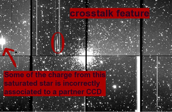
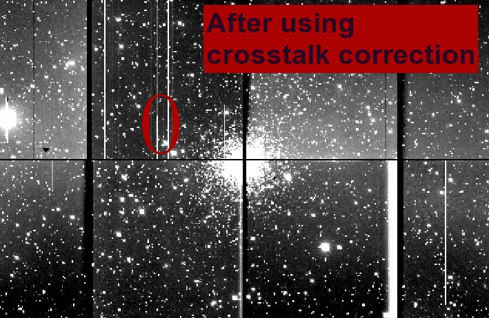
Crosstalk Correction Files

Crosstalk file for 8-channel mode [13], November 2010

Back To Mosaic II [14]

Updated: April 2010 by Andrea Kunder

Bad Pixel Mask for 8 channel mode

The Mosaic 2 CCDs have relatively few bad pixels, mostly around the edges and in CCD #3.

Bad pixels do not respond to light at all, or respond in a nonlinear way. These can be removed from data using a bad pixel mask. The current bad pixel mask in the mscred package is from 2001, so we recommend using the updated bad pixel mask found here.

[15]

[16]

You can create your own bad pixel mask by taking appropriate flat field observations, or download the most recent mask image below.

Bad Pixel Mask Correction Files

Bad Pixel Mask for 8-channel mode [17], 14 May 2010

How To Use The Bad Pixel Mask

The bad pixel masks are not trimmed. Hence, your images must not be trimmed in order to use them.

Here are the steps to use the bad pixel masks:

download the Bad Pixel Mask for 8-channel mode [17] in the same directory as the directory you are reducing your images in.

Use these commands to change the header of your images, so that the image header keyword "BPM" will point to the new bad pixel masks:

hedit *.fits[1] BPM CAL0510/bpm1_0510.pl veri- show+
hedit *.fits[2] BPM CAL0510/bpm2_0510.pl veri- show+
hedit *.fits[3] BPM CAL0510/bpm3_0510.pl veri- show+
hedit *.fits[4] BPM CAL0510/bpm4_0510.pl veri- show+
hedit *.fits[5] BPM CAL0510/bpm5_0510.pl veri- show+
hedit *.fits[6] BPM CAL0510/bpm6_0510.pl veri- show+
hedit *.fits[7] BPM CAL0510/bpm7_0510.pl veri- show+
hedit *.fits[8] BPM CAL0510/bpm8_0510.pl veri- show+

run "ccdproc"
here is an example:

images	=	@objects.list	List of Mosaic CCD images to process
(output	=	)	List of output processed images
(bpmasks	=	)	List of output bad pixel masks
(ccdtype	=	object)	CCD image type to process
(noproc	=	no)	List processing steps only?

(xtalkco	=	yes)	Apply crosstalk correction?
(fixpix	=	yes)	Apply bad pixel mask correction?
(oversca	=	yes)	Apply overscan strip correction?
(trim	=	yes)	Trim the image?
(zerocor	=	yes)	Apply zero level correction?
(darkcor	=	no)	Apply dark count correction?
(flatcor	=	yes)	Apply flat field correction?
(sflatco	=	no)	Apply sky flat field correction?
(split	=	no)	Use split images during processing?
(merge	=	no)	Merge amplifiers from same CCD?

(xtalkfi	=	xtalk090401.txt)	Crosstalk file
(fixfile	=	BPM)	List of bad pixel masks
(saturat	=	)	Saturated pixel threshold
(sgrow	=	1)	Saturated pixel grow radius
(bleed	=	20000.)	Bleed pixel threshold
(btrail	=	15)	Bleed trail minimum
(bgrow	=	1)	Bleed pixel grow radius
(biassec	=	!biassec)	Overscan strip image section
(trimsec	=	!trimsec)	Trim data section
(zero	=	Zero.fits)	List of zero level calibration images
(dark	=	)	List of dark count calibration images
(flat	=	Dflat.fits)	List of flat field images
(sflat	=	Sflat.fits)	List of secondary flat field images
(minrepl	=	1.)	Minimum flat field value

(interac	=	no)	Fit overscan interactively?
(functio	=	legendre)	Fitting function
(order	=	1)	Number of polynomial terms or spline pieces
(sample	=	*)	Sample points to fit
(naverag	=	1)	Number of sample points to combine
(niterat	=	1)	Number of rejection iterations
(low_rej	=	3.)	Low sigma rejection factor
(high_re	=	3.)	High sigma rejection factor
(grow	=	0.)	Rejection growing radius
(fd	=	)
(fd2	=	)
(mode	=	ql)

Generate Your Own Bad Pixel Mask

Take Data: 7 Bias images, 7 Domeflats with short exposure times, 7 Domeflats with long exposure times.
(The [OIII] filter works well to allow for a large dynamic range without using exposures that are too short. With the [OIII] filter you can take about 50s and 5s exposures.)

Zerocombine the Biases

Bias subtract the Domeflats

Flatcombine the domeflats with long exposure times

Flatcombine the domeflats with short exposure times

Divide the short exposure dome flat by the long exposure dome flat.
(The iraf command to use is "mscarith")

download an old Mosaic bad pixel mask to use as a starting template

Display an image with the bad pixel mask overlayed:

mscred> display DividedFlat.fits[1] 1 overlay=bpm1_0102.pl

Visually inspect the image and find bad pixels. Add these bad pixels to the bad pixel mask:
imreplace bpm1_0102.pl[431:431,2631:2631] 1. (to indicate a bad pixel) and imreplace bpm1_0102.pl[334:334,1:4096] 1. (to indicate a bad column)

Back To Mosaic II [12]

Updated: May 2010 by Andrea Kunder