THIS INSTRUMENT HAS BEEN RETIRED. INFORMATION PROVIDED HERE IS FOR REFERENCE ONLY
|
The CTIO Mosaic II CCD imager was developed together with the Mosaic I in use on the KPNO Mayall 4-m and 0.9-m telescopes and replaces the BTC camera previously used at prime focus on the V. M. Blanco 4-m telescope. Mosaic II will be retired in 2012 when it will be replaced by The Dark Energy Camera [1] (DECam).
Detector: 8 2048x2048 SITe CCDs
|
 |
| Andrea Kunder | : akunderATctio.noao.edu | Primary contact |
| Sean Points | : spointsATctio.noao.edu | |
| Alistair Walker | : awalkerATctio.noao.edu | |
| Chris Smith | : csmithATctio.noao.edu | |
| Tim Abbott | : tabbottATctio.noao.edu |
Last updated: 9 August 2012
CTIO Mosaic Support Pages [12] (internal use only)
4-m MOSAIC II CCD Imager COOKBOOK
A. Kunder 2010, modified from K. Olson 2003
DON'T PANIC !!
Three windows that look like the images below should be on your screen. These are virtual desktops. ctioa0 runs the camera electronics and ctioa8 accepts and stores the images. Do not use the observing desktop for anything other than taking observations! (Why? The observing desktop runs on ctioa1, which is a very old machine. Your data are transferred to ctioa8 automatically by the DCA. If you type e.g. "display obj001.fits 1" in the Arcon window, you are asking ctioa1's slooow CPU to display an image that it accesses across the network. Bad idea!).
The following images show the VNC windows:
 [13]
[13]
 [14]
[14]
Typing "lpar obspars" will list the contents of obspars, for example, while simply typing "obspars" or "epar obspars" will allow you to edit the values. The exception to this last statement is detpars: to edit detpars, DO NOT type "detpars" or "epar detpars"--you must instead type "setdet force+", so as to ensure that your changes are updated in the instrument.
"mscdisp test zrange- zscale - z1=1000 z2=50000"
Calculate the offset needed to bring the star to the center (the pixel scale is 0.27 arcsec/pix), by then typing
"zpt"
Then move the mouse on the center of the star and hit the space bar. The teloffset values will be read out in the xgterm. You can have the night assistant do this offset, or you can do it yourself by typing
"teloffset RA_offset_arcsec DEC_offset_arcsec"
command in the Arcon Aquistion box. Bear in mind that DEC increases with X and RA with Y. Take another 1-second test to verify that you moved the telescope in the right direction, and by the right amount.
"settemp"
--this command reads the temperature of the upper truss and records it in the "temperature" parameter of instrpars, described above. It also takes a guess at the best focus value--use this value as the focus value of the middle of your sequence. Now type
"focus"
specify an exposure time of 5-15 sec, and use the R filter (if you use another filter to do the focus, bear in mind that Arcon will add the focus offset listed in wheel1 to the focus when taking an exposure). Using the parameter values specified in telpars, Arcon will now take a sequence of N exposures, stepping the focus and shifting the charge by a number of rows between each one. After the exposure is done reading out, you will see an image containing columns of stars on the RTD. It will look something like this and like this if you zoom in.
In an IRAF window on ctioa8, type
"mscfocus"
You will now select stars to use in calculating the best focus. Place the cursor on the top star in a cleanly separated, unsaturated sequence and type the "g" key (always use the top star, regardless of whether or not there is a double step between it and its neighbor). A window will appear displaying the FWHM as a function of focus for that star. Type "q", place the cursor on the top star of another column, and type "g" again. Repeat this sequence until you have measured the focus profiles of 1-2 stars on each CCD. With the cursor in the ximtool, finally type "q". You will now see a window overlaying the focus sequences for all of the stars you just measured. If there are strongly outlying points, place the cursor on them and type "d", which deletes the information for the whole star associated with that point, Once you are satisfied, type "q", and the program calculates the best focus for you.
In mscfocus, you might prefer to use the "m" key (again always use the top star). Hit the "m" key for stars in all the different CCDs. When you have sampled a sufficient quantity, hit "q". You will get something like this:
image here
Note the best focus value and fwhm, which is displayed on the top of the pop-up window.
Enter the best focus value in the "basefocus" parameter in instrpars, and change "reftemp" to equal the value in "temperature". If "setfocus" is set to "auto", Arcon will calculate the difference between "temperature" and "reftemp", multiply this by the temperature coefficient, and add it to "basefocus" before taking an image. Until you type "settemp" again, this focus adjustment will be 0. Later during the night, if you find that the temperature has changed significantly, type "settemp" before taking an exposure, and "temperature" will be updated.
If you don't like using "mscfocus", you can always use "mscexam" instead. "mscexam" works just like "imexam"--you can examine stars with the "r" or "e" key to pick which of the stars in the focus sequence is in best focus.
image here
then you must decrease the focus value. If the profile looks East-West, incrase the focus value.
image here
Back To Mosaic II [15]
detpars:
| (xsum = | 1) | pixels summed in X direction |
| (ysum = | 1) | pixels summed in Y direction |
| (ysize = | 8192) | Height of centered ROI (full width) |
| (pixsize = | 15.) | Pixel size in microns |
| (nxpixels = | 2048) | Detector size in X |
| (nypixels = | 4096) | Detector size in Y |
| (detname = | "Mosaic2") | Detector identification |
| (mode = | "ql") |
The detpars file is where you can specify binning, if you want it, and set regions of interest (ROIs). Note that setting ROIs does not lower the readout time as much as you would expect; talk to you staff contact before using ROIs. Also, as stated above, do NOT change the parameters in detpars by typing "detpars" or "epar detpars"; you MUST use "setdet force+".
instrpars
| filter1 = | "VR" | Filter in wheel one |
| (wheel1 = | "") | Filter info. pset for wheel one\n\n# SELECTING |
| (setfilters = | "yes") | Query and set filters?\n\n# SETTING FOCUS FOR E |
| (setfocus = | "auto") | Query and set focus? |
| (temperature = | 5.7) | Telescope truss temperature (C) |
| (basefocus = | 17600.) | Telescope focus base value |
| (reftemp = | 5.2) | Telescope temperature for base focus value (C) |
| (tfrcoefs = | "1 -135.0") | Coeficients of Temperature-Focus relationship\n |
| (tv1focus = | -6.203) | Focus for camera 1 |
| (tv2focus = | -2.499) | Focus for camera 2\n\n# SHUTTER READY POSITION |
| (shutter_read = | "auto") | Position of shutter when NOT exposing\n |
| (instrname = | "mosaic") | Instrument name |
| (mode = | "ql") |
In instrpars, the parameters of greatest concern to you will be "setfocus", "temperature", "basefocus", and "reftemp". By setting "setfocus" to "auto" (RECOMMENDED), you allow the telescope to update its focus for changes in temperature (using the coefficient in "tfrcoefs", where "1 -135.0" means a change of -135 microns of focus for a 1 degree change in temperature). This procedure is described in detail below, under the focus procedures. You should also normally leave "setfilters" to "yes", so that the Arcon will ask you for the filter whenever you take an exposure. The ONLY reason you would want to set it to "no" (in which case Arcon uses whatever filter is in "filter1"), is if your program uses only one filter.
epar obspars
obspars:
| picture = | 1001 | Picture number of first exposure |
| (template = | "") | Image name template |
| (autopicnum = | yes) | Generate picture number automatically ? |
| (detupdate = | yes) | Update detector parameters automatically ?\n\n# |
| (postpic = | "") | Post processing command for single picture |
| (postseq = | "") | Post processing command for sequences |
| (restart = | yes) | Restart the server on every command ?\n\n# ADDI |
| (observers = | "Galvez, Bonati") | Observers |
| (propid = | "007") | Observing proposal ID |
| (comments = | "") | (comments = " ") |
| (comfile = | "") | Observer header comments file\n |
| (mode = | "ql") |
What might you want to change in obspars? The fields "observers", "propid", and "comments" are all added to the header and to the automatic observing logs, and should correspond to your program. If you leave "template" blank, then your images will have our standard prefixes ("obj" for objects, "dflat" for dome flats, "zero" for biases, "sflat" for sky flats, and "focus" for focus frames) plus the picture number given by "picture" (which is automatically incremented for you as long as "autopicnum" is set to "yes"). Some observers like to use one template for all types of exposures, which they enter in the "template" field. It's also popular to change the "picture" number at the beginning of each night (say 1001 for the first night, 2001 for the second, etc.) so as to easily distinguish images taken on different nights.
telpars:
| telfocus = | 158211 | Telescope focus |
| nfexpo = | 7 | Number of focus exposures |
| freference = | 17500 | Focus value |
| fdelta = | 100 | Focus increment |
| (ra_offset = | 0.) | RA Offset (arcsec) |
| (dec_offset = | 0.) | Declination Offset (arcsec)\n\n# PARAMETERS FOR |
| (fnrows = | 30) | Focus number of rows to reverse shift |
| (refis = | "middle") | Reference is first, middle or last ex\nposure? |
| (focmode = | "auto") | Focus mode\n\n# FOR INFORMATION ONLY |
| (telname = | "ct4m") | Telescope name |
| (station = | "pf") | Focal station |
| (fratio = | "f/2.9") | Focal ratio |
| (platescale = | 18.) | Plate scale (arseconds/mm) |
| (mode = | "ql") |
The current telescope focus is stored in telpars (do not change "telfocus" by hand, as it is updated automatically as long as "setfocus" in instrpars is set to "yes" or "auto"), as are the parameters that control how focus sequences are taken. Depending on the seeing, you may want to change the focus step ("fdelta") between successive exposures in a focus sequence, or the number of focus exposures in a sequence ("nfexpo"). The values listed above are good all-purpose values.
wheel1:
| (id1 = | "U") | Short identifier for filter in position 1 |
| (name1 = | "U c6001") | Full name of filter in position 1 |
| (focus1 = | -200.) | Focus value for filter 1 \n |
| (id2 = | "B") | Short identifier for filter in position 2 |
| (name2 = | "B Harris c6002") | Full name of filter in position 2 |
| (focus2 = | 10.) | Focus value for filter 2 \n |
| (id3 = | "V") | Short identifier for filter in position 3 |
| (name3 = | "V Harris c6026") | Full name of filter in position 3 |
| (focus3 = | 30.) | Focus value for filter 3 \n |
| (id4 = | "R") | Short identifier for filter in position 4 |
| (name4 = | "R Harris c6004") | Full name of filter in position 4 |
| (focus4 = | 0.) | Focus value for filter 4 \n |
| (id5 = | "I") | Short identifier for filter in position 5 |
| (name5 = | "I c6028") | Full name of filter in position 5 |
| (focus5 = | 0.) | Focus value for filter 5 \n |
| (id6 = | "z") | Short identifier for filter in position 6 |
| (name6 = | "z SDSS c6020") | Full name of filter in position 6 |
| (focus6 = | -15.) | Focus value for filter 6 \n |
| (id7 = | "M") | Short identifier for filter in position 7 |
| (name7 = | "M Washington c6007") | Full name of filter in position 7 |
| (focus7 = | 65.) | Focus value for filter 7 \n |
| (id8 = | "D51") | Short identifier for filter in position 8 |
| (name8 = | "DDO 51 c6008") | Full name of filter in position 8 |
| (focus8 = | -35.) | Focus value for filter 8 \n |
| (id9 = | "VR") | Short identifier for filter in position 9 |
| (name9 = | "VR SuperMacho c6027") | Full name of filter in position 9 |
| (focus9 = | 30.) | Focus value for filter 9 \n |
| (id10 = | "o3") | Short identifier for filter in position 10 |
| (name10 = | "o3 OIII c6014") | Full name of filter in position 10 |
| (focus10 = | 130.) | Focus value for filter 10 \n |
| (id11 = | "g") | Short identifier for filter in position 11 |
| (name11 = | "g SDSS c6017") | Full name of filter in position 11 |
| (focus11 = | 30.) | Focus value for filter 11 \n |
| (id12 = | "r") | Short identifier for filter in position 12 |
| (name12 = | "r SDSS c6018") | Full name of filter in position 12 |
| (focus12 = | 120.) | Focus value for filter 12 \n |
| (id13 = | "i") | Short identifier for filter in position 13 |
| (name13 = | "i SDSS c6019") | Full name of filter in position 13 |
| (focus13 = | -20.) | Focus value for filter 13 \n |
| (id14 = | "u") | Short identifier for filter in position 14 |
| (name14 = | "u SDSS c6021") | Full name of filter in position 14 |
| (focus14 = | 230.) | Focus value for filter 14 \n |
| (first_pos = | 1.) | First Filter positions in wheel (read only) |
| (last_pos = | 14.) | Last Filter positions in wheel (read only) |
| (mode = | "ql") |
The wheel1 parameter file contains all of the information about the filters: their short identifiers (the name you type when requesting that Arcon use a certain filter, and the name that appears on the GUI), their full names, and their focus offsets with respect to the R filter. The focus offset is applied automatically when taking an exposure; Arcon assumes that the base focus value that appears in instrpars (see above and the section on the focus procedure) corresponds to the R filter. Normally, you should not need to change anything in the wheel1 parameter file; we recommend, however, that you check to make sure that the focus offsets are set to the measured values listed on the filter page [2].
Taken on the engineering night of August 3 1999, by R. Schommer, C. Smith, R. Smith.
Click on the pictures for full frame versions
 [22]
[22]
Figure 1: 10 sec V band exposure of Galactic nebula M8
 [23]
[23]  [24]
[24]
Figure 2: 10s and 180s Halpha exposures of the M16 nebula.
 [25]
[25]
Figure 3: 20 sec V band exposure on Baade's Window. Clusters are NGC 6522 and 6528.
 [26]
[26]
Figure 4: 500 sec V band exposure of NGC 6822 Local Group dwarf galaxy.
Here are some test data for the Mosaic II CCDs, as measured by Tom Wolfe in the NOAO/Tucson CCD Lab. All have excellent CTE, dark rate less than 1 e-/pix/hour at -90C, and charge injection of 1-2 electrons if a reverse vertical clear is done prior to integration. When reading the QE figures, remember that the 4-m prime focus corrector does not transmit below 3300A.
| CCD# | 21 | 22 | 25 | 26 | 27 | 28 | 29 | 31 |
| Gain e-/adu (8 us ) Amp A: | 2.18 | 2.34 | 1.72 | 1.78 | 1.70 | 1.70 | 1.63 | 1.85 |
| Gain e-/adu (8 us ) Amp B: | 1.78 | 2.23 | 1.78 | 1.73 | 1.69 | 1.64 | 1.68 | 1.73 |
| Noise e-(8 us dwell) Amp A: | 5.4 | 5.4 | 3.8 | 4.0 | 4.0 | 4.1 | 3.4 | 4.4 |
| Noise e-(8 us dwell) Amp B: | 4.8 | 5.7 | 4.7 | 4.6 | 4.4 | 4.0 | 4.2 | 3.5 |
| Fullwell Ke-: | 90 | 69 | 82 | 80 | 63 | 64 | 63 | 83 |
| QE % at 3000A: | 9 | 8 | 9 | 9 | 8 | |||
| QE % at 3340A: | 18 | 19 | 18 | 17 | 18 | 18 | 17 | |
| QE % at 3650A: | 48 | 51 | 44 | 49 | 46 | 48 | 48 | 46 |
| QE % at 4050A: | 65 | 69 | 72 | 69 | 65 | 69 | 67 | 69 |
| QE % at 6000A: | 82 | 85 | 89 | 88 | 84 | 88 | 86 | 85 |
| QE % at 8000A: | 61 | 70 | 71 | 70 | 69 | 68 | 69 | 70 |
| QE % at 9000A: | 37 | 42 | 40 | 53 | 41 | 39 | 39 | 41 |
| QE % at 10000A: | 13 | 10 | 11 | 11 | 11 | 11 | 12 | |
| # of full column defects: | 0 | 2 | 1 | 1 | 2 | 0 | 1 | 0 |
| # of partial column defects: | 1 | 2 | 0 | 9 | 1 | 0 | 6 | 0 |
Full frame, unbinned, dual readout
| CCD (1) | 1a | 1b | 2a | 2b | 3a | 3b | 4a | 4b |
| FITS section | 1 | 2 | 3 | 4 | 5 | 6 | 7 | 8 |
|
Gain (e-/ADU) 22 Nov 2000 (2) |
2.5 | 2.8 | 2.5 | 2.2 | 2.4 | 2.4 | 2.4 | 2.3 |
|
Gain (e-/ADU) 17 May 2002 (2) |
2.75 | 2.86 | 2.84 | 2.30 | 2.45 | 2.37 | 2.53 | 2.37 |
|
Gain (e-/ADU) 08 May 2004 (6) |
2.73 | 2.91 | 2.83 | 2.27 | 2.86 | 2.52 | 2.42 | 2.36 |
|
Gain (e-/ADU) Oct 2005 (2, 7) |
2.81 | 2.95 | 2.88 | 2.34 | 2.9 | 2.56 | 2.56 | 2.39 |
|
Read noise (e-) 22 Nov 2000 |
5.9 | 7.2 | 6.5 | 5.0 | 8.6 | 11.5 | 8.1 | 6.8 |
|
Read noise (e-) 17 May 2002 (3) |
5.97 | 9.4 | 7.0 | 5.06 | 7.1 | 10.0 | 8.3 | 6.2 |
|
Read noise (e-) 08 May 2004 (6) |
5.79 | 5.63 | 6.17 | 4.68 | 8.78 | 8.10 | 5.78 | 4.99 |
|
Read noise (e-) Oct 2005 (7) |
6.25 | 8.66 | 6.98 | 5.23 | 10.02 | 8.79 | 6.75 | 6.07 |
|
Nonlinearities 17 May 2002 (4) |
~<1% | ~<1% | ~<1% | ~<1% | ~<1% | ~<1% | ~<0.8% | ~<1% |
|
Nonlinearities Oct 2005 (4) |
~<1% | ~<1% | ~<1% | ~<1% | ~<1% | ~<1% | ~<1% | ~<1% |
|
Spurious Charge (ADU) 17 May 2002 (5) |
N/M | ~10 | ~5 | ~8 | ~10 | ~12 | ~15 | ~8 |
|
Full well (e-) 08 May 2004 (6) |
130,000 | 125,000 | 91,000 | 87,000 | 77,000 | 81,000 | 70,000 | 71,000 |
|
Full well (e-) Oct 2005 (7) |
>112,000 | >118,000 | 86,000 | 89,000 | 87,000 | 97,000 | 67,000 | 67,000 |
| CCD (1) | 5b | 5a | 6b | 6a | 7b | 7a | 8b | 8a |
| FITS section | 9 | 10 | 11 | 12 | 13 | 14 | 15 | 16 |
|
Gain (e-/ADU) 22 Nov 2000 (2) |
2.0 | 1.8 | 2.1 | 2.0 | 2.5 | 2.6 | 3.3 | 3.3 |
|
Gain (e-/ADU) 17 May 2002 (2) |
2.03 | 1.95 | 2.24 | 2.13 | 2.63 | 2.79 | 3.35 | 3.49 |
|
Gain (e-/ADU) 08 May 2004 (6) |
2.01 | 1.93 | 2.25 | 2.13 | 2.17 | 2.38 | 2.69 | 2.60 |
|
Gain (e-/ADU) Oct 2005 (2, 7) |
2.01 | 1.99 | 2.22 | 2.13 | 2.17 | 2.39 | 2.66 | 2.77 |
|
Read noise (e-) 22 Nov 2000 |
7.6 | 7.0 | 8.3 | 7.2 | 5.0 | 5.6 | 7.7 | 7.6 |
|
Read noise (e-) 17 May 2002 (3) |
7.1 | 6.8 | 14.6 | 8.1 | 6.05 | 8.1 | 8.7 | 8.7 |
|
Read noise (e-) 08 May 2004 (6) |
5.23 | 5.49 | 5.85 | 5.73 | 4.35 | 5.17 | 5.90 | 6.08 |
|
Read noise (e-) Oct 2005 (7) |
7.22 | 10.23 | 15.1 | 8.89 | 6.94 | 6.42 | 9.05 | 8.56 |
|
Nonlinearities 17 May 2002 (4) |
~<1% | ~<1% | ~<1% | ~<1% | ~<1% | ~<1% | ~<1% | ~<1% |
|
Nonlinearities Oct 2005 (4) |
~<1% | ~<1% | ~<1% | ~<1% | ~<1% | ~<1% | ~<1% | ~<1% |
|
Spurious Charge (ADU) 17 May 2002 (5) |
~-5 | ~-5 | ~-5 | ~-5 | ~-2 | ~-2 | ~-5 | ~-5 |
|
Full well (e-) 08 May 2004 (6) |
76,300 | 84,000 | 97,000 | 102,000 | 95,500 | 93,000 | 62,000 | 67,600 |
|
Full well (e-) Oct 2005 (7) |
76,000 | 80,000 | 73,000 | 81,000 | 91,500 | 100,000 | 56,000 | 61,000 |
1. When looking at a Mosaic image, the 8 lower segments are denoted from left to right (ccd,amp) 1a,1b,2a,2b,3a,3b,4a,4b. Across the top, from left to right: 5b,5a,6b,6a,7b,7a,8b,8a.
2. Gain measured from Transfer curve.
3. Read noise calculated from standard deviation of a bias frame × gain.
4. Nonlinearities are the width of the envelope of the count rate curve over a large part of the dynamic range of the detector. They include any variation in the light source and shutter effects, although the shutter delay has been removed to first order. These measurements are therefore an upper bound.
5. Spurious charge is charge that is injected into the CCD as a result of parallel clocking. It shows up as a slope in the bias level in the vertical direction, quoted here in ADUs from the top to the bottom of the unbinned image.
6. Measured in the La Serena lab after the installation of a new CCD #3. Full well was determined from the variance curve, noise from the overscan.
7. Measured in situ at Blanco prime focus, using flat field lights.
Gain, Read Noise, and Full Well of Mosaic II CCDs reading in 8 channel (8a) mode.
Last updated: 31 August 2000
| Chip 1 | Chip 2 | Chip 3 | Chip 4 | Chip 5 | Chip 6 | Chip 7 | Chip 8 | |
| Gain (e-/adu) |
2.6 | 2.7 | 2.3 | 2.4 | 1.8 | 2.0 | 2.7 | 3.3 |
| Read Noise (e-) |
6.1 e- | 7.8 e- | 7.9 e- | 7.8 e- | 7.1 e- | 8.0 e- | 5.8 e- | 7.7 e- |
| Full well (adu) |
48000 | 34500 | 28000 | 29000 | 43500 | 52000 | 41000 | 21500 |
based on KPNO Mosaic I Manual by
Taft Armandroff, Todd Boroson, Jim De Veny, Steve Heathcote,
George Jacoby, Tod Lauer, Phil Massey
Rich Reed, Frank Valdes, David Vaughnn
originally February 5,1999
CTIO VERSION
February 2000
edited by R. Schommer, C. Smith, K. Olsen, and A. Walker
[send comments on manual to awalkerATnoao.edu and csmithATnoao.edu]
| Arrays | : 8 2048x4096 SITe CCDs; thinned , science grade |
| Image size | : 8192 x 8192 @ 16 bits, plus header, overscan:~135 Mbytes |
| Pixels size | : 15-um (0.27"/pixel at the 4-m) |
| Read-noise | : ~6 -8e-, very low fixed pattern noise |
| DQE | : 86% peak at 6000Å (average for 8 CCDs; see also Figure 3.1.2) |
| Dark-current | : ~ <2 e-/pixel/hr; but charge injection introduces a ramp of about 10-12 electrons; needs to be taken out with a summed zero exposure. |
| Read-out time | : 2.5 minutes in 8 channel mode; expected ~100sec in 16-channel mode |
| CCD Gaps | : ~0.7 mm (~50 pixels) in rows; ~0.5 mm (~35 pixels) in columns |
| Cosmetics | : Good to excellent: typically 2 bad columns per CCD, but many 2-8 pixel areas of 5% variation (flatfield completely) and some very large areas of 10% variations that all flatfield to <0.5% |
| Filters | : 5.75"x5.75"; almost parfocal, 15 filters now available (UBVRI; see Sec 2.6) |
| Saturation | : Typically, linear to 0.1% to 70,000 e- |
| Gain | : ~2 e-/ADU |
| Count Rates | : At UBVRI=20th mag: U: 35; B:330; V: 340; R: 410; I: 225 e-/sec |
| FOV | : 36'x36', XIMTOOL Orientation: North- right, East-up |
| Scale | : 0.27"/pixel at center; decreases quadratically by 6.5% out to corners |
| Image quality | : PSF reasonably constant across the FOV, but ~6% larger in linear scale at the corners. Focussing on a star approx halfway to the corner of the array gives a slightly more even image quality over the whole field, however the focal plane is not tilted wrt to the CCDs, and focus at center is only around 30 microns less than the outer parts of the array. to corner. |
| Artifacts | : No obvious filter ghosts; electronic crosstalk between pairs of CCDS at ~0.1% and can be removed accurately when reducing the data |
| Typical focus | : 14500 at ~15C ; change with temperature: -135 units per degree C |
| ADC: | : Atmospheric Dispersion Correction: Use ADC in "ENABLED" mode via the operators's TCS console. Provides continuous trackinge except for zenith distances less than 8 degrees, where it returns to its nominal position |
Acquisition commands are given on computer named ctioa0
Analysis commands are given on computer named ctio4m
| enable | enable or disable filters/motors/some TCS functions |
| motor init | initialize the filters, including the name assignments |
| motor stat | list of status of motors, including filter assignments and position |
| setdet | change detector parameters (careful!) |
| instrpars | change instrument parameters (careful!) |
| telpars | change telescope parameters (careful!) |
| obspars | change observing parameters |
| observe | take one or more exposures prompting for the exposure type |
| doobs | a script which takes flats/objects for a list of filters |
| mosdither | takes N (typically 3-5) dithered images in a single filter to fill the gaps in array. Dither patterns are stored (by default) in /u4m2/mosaic/dithers |
| more | take more exposures just like the last one |
| test | take a test exposure. The output image, test, is overwritten each time |
| object | take one or more object exposures |
| zero | take one or more zero (bias) exposures |
| dark | take one or more dark exposures |
| dflat | take one or more dome flats |
| pflat | take one or more projector flats |
| sflat | take one or more sky flats |
| focus | take a focus frame |
| snap | take a binned exposure for quick readout |
| settemp | pokes serrulier truss temperature into instrpars |
Exposure Control Commands
| pause | pause exposure (e.g. clouds) [do not ABORT or STOP from within pause!] |
| resume | resume a paused exposure [then ABORT or STOP if necessary!] |
| tchange | increase or decrease the exposure time |
| stop | stop an exposure (and sequence of exposures) reading out the detector |
| abort | abort an exposure (or sequence) discarding the data |
| pictitle | change the title of the picture |
| mscdisplay | display an entire mosaic frame |
| mscexamine | general tool for examining images |
| mscwfits | write mosaic frames to tape in multi-extension FITS format |
Tape your data as you go>; DLT-7000 (~250 images/tape), DDS3(~80 images/tape), and Exabyte drives (~35 images/tape) are available. Write time: ~55 seconds/image to DLT, ~90seconds/image to DDS3,~3 minutes/image to Exabyte. You are expected to be off the computer by noon of your last day!
You can buy DLT, DDS3 and Exabyte tapes on Tololo, but bringing your own is cheaper.
Take dome flats and/or twilight flats. Dome flats may show slopes across the Mosaic with amplitude of a few percent, twilights are better (1%) although we are not sure if an "artifact" in the south-west corner has gone away. The long read time makes taking twilight flats a real challenge, don't expect to get more than 6 or 7 at a time. For really flat images you'll need to flatten using dark-sky frames combined and filtered to remove stars. You may be able to use your object frames or fields (preferably with not too many bright stars) taken for the purpose. Remember bright stars bleed east-west, and you should jog at least 30 arcsec and preferably more.
Take dark exposures of similar length to your science exposures, note that the general dark level is zero and hot pixels are usually non-linear, so this is really only for the truly paranoic.
Take zeroes (i.e., biases) too -- Be sure that the dome is dark for darks and zeroes! The instrument is reasonably light tight but we do operate with the cage doors removed, so bright lights are not a good idea.
It's a good idea to take a careful look at your calibration frames individually, before combining. And remember that some of the CCDs have very considerable slopes and variations as you go up the overscan, so fitting the overscan with a constant or line may not be appropriate.
CAUTION: The Mosaic 2 camera allows 2x2 to 4x8 binning although not fully tested for science frames reductions.
This page was last updated on Feb 22, 2000 by ARW
The NOAO CCD Mosaic is a wide field imager having 8192 x 8192 pixels. At the 4m, where the pixels are 0.27" on the sky, this provides a field of view of 36.8 arcmin on a side.
The CCDs are read in ~2.5 minutes through 4 Arcon controllers to a data taking computer (currently known as ctioa0), which serves as an intermediary data gateway. The pictures really end up on a much faster computer (ctio4m) where you can display and examine the data, perform full reductions, and tape the data much more effectively. Ctioa0 should be used only to do the minimal work required to take observations because the data rate through it is tremendous and nearly pegs the CPU at 100%.
Pictures are 135 Mbytes each. A typical night of ~70 pictures produces about 10 Gbytes. Be aware that processing this data, even just reading it, is a major task for the computing systems that most astronomers have access to. We recommend using a DLT tape drive (our DLT 7000 will write the lower density and cheaper DLT 4000 cassettes if you prefer, although currently there is a problem with the low density mode); however, we provide Exabyte 820 (8505XL compatible) and DDS3 drives for those who do not have DLTs. Provide enough time to tape your data each night. With the Exabytes, a picture takes 3 minutes to tape, so 70 pictures will take nearly 4 hours even without a verification pass. DDS3 writing with mscwfits take about 90s for each image , and the DDS3 tapes hold 12Gbytes (uncompressed). To summarize, DLT IV TAPE + DLT7000 drive holds 35 GB and writes one 135 MB image in 50 seconds.
The Mosaic requires large (5.75 inch) filters to avoid vignetting. We can provide an adapter for 4 inch filters, but using them makes poor use of the Mosaic's wide-field.
Despite the data volume and the unusual computer arrangements, using the Mosaic is still not very different than observing with our other CCD systems.
This manual is intended for an observer planning to use the NOAO CCD Mosaic imager. It is not intended to serve as a hardware or software reference document describing the inner working of Mosaic, although some details at that level may appear to help the observer plan observing strategies. Also, we assume that the observer is already familiar with CCD cameras, observations, and data reductions.
Two very brief summary pages are at the front of this manual. If you've read this far, and don't plan to read any further, be sure you understand those 2 pages.
This manual is an edited version of the KPNO manual, kindly made available by G. Jacoby. We have adopted bald-faced plagarism as our philosophy, and kept the structure and much of the text of that document. We have made changes were the systems are clearly different or where we have direct measures relating to the performance of our system. We will update this version as improved information becomes available.
Development of the Mosaic system is a continuing process, although only very minor adjustments are being made at this time. Throughout the lifetime of the instrument, filters will be added, old ones replaced, and software enhanced. This manual represents the status as of the date on the cover page. We expect to revise the manual occasionally to include information gained during engineering runs, as well as to reflect new filters.
Other useful information regarding the use of Mosaic, CCDs, and observing and reduction software can be found at:
Direct Imaging Manual (http://www.noao.edu/kpno/manuals/dim/ [28])
Mosaic Web Pages (http://www.noao.edu/kpno/mosaic/mosaic.html [5])
Various Publications (SPIE, ADASS, ...)
Mosaic Data Handling System (Valdes 1998, SPIE 3355, 497) (http://www.noao.edu/noao/meetings/spie98/mdhs.ps [29])
CCD Detector upgrade for NOAO's 8192 x 8192 Mosaic (Wolfe 1998, SPIE 3355, 487) (http://www.noao.edu/noao/meetings/spie98/wolfe.html [30])
What is better than an 8K x 8K Mosaic? (Muller 1998, SPIE 3355, 577) (http://www.noao.edu/noao/meetings/spie98/muller.ps [31])
This section was last updated on August13, 1999
| Hardware Contents: | |
| 1. | The Mosaic CCD |
| 2. | The Dewar |
| 3. | The Arcon Controllers |
| 4. | The CCD Shutter |
| 5. | The Filter Track |
| 6. | Filters for Mosaic |
| 7. | Operation of the Guider TVs |
| 8. | Correctors |
| 9. | Atmospheric Dispersion Corrector |
The Mosaic Imager features eight 2048 (serial or pixels/row) x 4096 (parallel or pixels/column) 15 m pixel CCDs arranged as an 8192 x 8192 pixel detector. The CCDs are read out through a single amplifier per chip simultaneously to 8 controller inputs (on 4 Arcon controllers). The resulting mosaic array is a square about 5 inches on an edge. The gaps between CCDs are kept to about 0.7 mm in the row direction and 0.5 mm in the column direction. [see Figure 3.1.1 showing an image labeled with chip numbers.] We have populated the Mosaic Imager with thinned, AR coated SITe CCDs. These chips have only minor flaws which have little effect on their scientific performance, but they do require careful calibration to attain excellent flat-fielded images. Please see current CCDs [16] for some characteristics of the Mosaic II chips.
Figure 3.1.1: A Flat-field (R band) map of the CCDs in Mosaic I
with their "extensions" (im1, im2, im3, ...) as used in the IRAF nomenclature (see section 5).
Figure 3.1.2: The average QE for the 8 SITe CCDs in Mosaic I.
Figure 3.1.2 shows the average QE for the 8 CCDs at KPNO. Individual CCDs may deviate from this curve as shown in Figure 3.1.3.

Figure 3.1.3: The QE differences relative to the average for the 8 SITe CCDs in Mosaic I.
Also shown are the readnoise (RN) and gain (GN) values for each CCD.
The Mosaic dewar is a large (6.3 liter) vacuum vessel radiatively coupled to the CCD mount. It is the large round cylindrical object in the center of Figure 3.2.1. The hold time of the dewar is 18 hours. It will be filled by an observing technician at the start and end of each night.
Several temperatures within the dewar are monitored and displayed in the Mosaic Graphical User Interface (GUI). The CCDs should be between -95and -105C. The dewar tank is cooled to -166 C or cooler. A good way to detect the exhaustion of LN2 is the warming of the "fill neck" temperature, which is normally near 0 C. If this temperature begins to rise much above zero or any of the temperature boxes turn red, call for assistance to have the dewar filled.
Figure 3.2.1: The Mosaic system mounted at the back of the 0.9-m telescope at KPNO.
The dewar containing the 8 CCDs is the silvery, cylindrical object in the middle. It is surrounded by the filter track which is housed in the large black oval that extends horizontally across most of the picture.
The eight CCDs are read out through four Arcon controllers. These controllers run at 100 kpix/sec per CCD, yielding a readout time of ~2.5 minutes (in the single amplifier mode) and complete the transfer to disk on the data reduction computer. Data values are stored as 16-bit unsigned integers. For further details about the Arcon controller systems, see the technical paper by Roger Smith (http://www.ctio.noao.edu/instruments/arcon/arcon.html [32]).
The data taking computer (ctioa0) is a 125 Mhz Sun Sparcstation 10 running SunOS. It has sufficient resources to manage the data acquisition, but not much more. The large data volume is handed off to the reduction computer (ctio4m) via fast Ethernet for all analysis and reductions, thereby relieving the data taking machine of unnecessary loads. The reduction computer is a fast Sun Ultra with >45 Gbytes of disk and >512 Mbytes of RAM.

Figure 3.3.1: A view of the Mosaic system indicating 2 of the 4 Arcon controllers.
Also the south guide TV housing can be seen, as well as the large Mosaic dewar.
The shutter consists of a pair of opposing sliding blades, one of which has rectangular slots open for the guide field. The blades are attached to pneumatically driven cylinders to provide very fast control of the shutter. This design allows the TV guide fields to be shuttered independently of the science field. In the guide mode, the closed shutter still allows the TV guide cameras to see the sky. In the dark mode, these fields are closed as well. The acquisition software controls which mode the shutter remains in between exposures. For object observations, the shutter goes to the guide mode before the exposure begins. For requested observation types of dark, flat, or zero, the shutter goes to the dark mode before the exposure begins (and remains in this mode after the exposure and readout are completed). Note that the TV fields are always open when the shutter is open; the different shutter modes only control the TV fields when the science shutter is closed. If you have been taking darks, flats, or zeros, you may need to set the shutter mode to guide in order to get light to the TV guide camera.
The time for the blades to move completely across the field is 23 msec. The motion of the blades during both opening and closing are in the same direction so that the exposure level is nearly constant over the array. The motion of the shutter blades is along columns. All exposure times are shorter than the nominal time requested, in the mean, by 22 milliseconds (measured May 31 2000), ie if you request a 2 second exposure the time is really 1.978 seconds. The nom-uniformity of exposure is approximately +/- 5 milliseconds. Thus you can do short exposures (eg 1 second), particularly if you take account of the 22 millisecond offset. A one second flat field exposure will have a +/- 0.5% percent non-uniformity du to shutter shading. A caveat is that we do not have data to test whether there is any temperature effect (these measurements weer done at 11C) or changes with time, or inclination of the instrument (we were pointed at the white spot). So to be VERY safe, avoid exposures shorter than approx 5 seconds.
The filter track holds 14 filters. For each filter position, there is a filter for the CCD field, and two separate filters for the two TV fields. Separate filters are used so that a narrow bandpass science filter does not constrain the observer to find very bright guide stars. Normally, one would use clear (BK7) filters for the TV, but one can use a red filter to minimize moonlight or match the science filter more accurately. One might want to match the science filter, at least approximately, to minimize a guider drift. Even at the 4-m, residuals after the correction from the ADCare of order 0.1-0.2 arcsec. This, and all filter decisions, must be made ahead of time, as the filters can only be changed during the day by a qualified observing technician.
Adapters exist to allow the use of 4-inch-square filters in the Mosaic filter track. At the 4-m, the 4-inch filters illuminate approximately 5.5K X 5.5K pixels (46% of the total sky area).
The positioning of the filter track is highly repeatable. However, the acceleration of the track can occasionally dislodge dust particles between filter moves, particularly if intervening movements have turned the filter upside down. In all cases, the filter track software moves the track in the direction that minimizes the distance moved to reach the requested filter position.
In addition to the 14-position filter track, there is a manual slide that can hold a single filter of the same size (5.75 inches square). This may be used, for example, to hold a bandpass filter when polarization filters are used in the track. Use of this ìhand-insert filterî changes the focus. At the 4-m, changing, inserting, or removing this filter can only be done at the maintenance (Northwest Annex) position.
Physical Dimensions: To fully utilize the field of view of the 8Kx8K, filters must be 5.75 inches (146 mm) square, and have 5.43 inches (138 mm) clear aperture. The optimum thickness that preserves image quality over the entire field of view is 0.47 inches (12.0 mm). All NOAO mosaic filters adhere to these specifications to maintain an approximately parfocal condition. We have determined focus offsets for some of the filters, and will enter more when we measure them. You also may want to tweak the TV camera focus (watch the FWHM graph on the PC Guider GUI) if your focus change is more than (say) 50 microns.
Currently available filters and Offsets: MOSAIC FILTER LIST [33]
Transmission curves: See Figures 3.61, 3.62, and 3.63 for plots of the current KPNO broad-band, H, and [OIII] filter transmission curves. ASCII Tables [34] that numerically describe the transmissions are available on the Mosaic Web Pages.
Figure 3.6.1: The broad band filter set, including the "White" and Gunn Z' filters.
The U-band filter is based on the same formulation as our 4" filter set (liquid CuSO4 + UG-1).
Figure 3.6.2: The current set of H-alpha (plus redshifted) filters. Note that H-alpha+16 serves as a [SII] filter.
Figure 3.6.3: The current [OIII] filter available for Mosaic.
It will be replaced soon with one that is slightly blue-shifted, for improved performance at the 0.9-m
Figure 3.6.4: The [OIII] off-band filter available for Mosaic.
Figure 3.6.4: The V-band filter installed in the filter track.
The 2 TV guider filters are visible to the lower left and upper right of the science filter. An Arcon controller can be seen in the background to the right.
Guiding with the Mosaic is accomplished using one of two TV cameras on the north and south sides of the science field. These are intensified fiber-optically coupled CCD cameras ("ICCDs"), and so, they can be damaged if exposed to bright light. The video signal from the selected TV camera is fed to the leaky guider system. [35] The field of view of each camera is about 2.2 arcmin on a side at the 4-m.
The TVs field of view is fixed with respect to the science field. At the 4-m, the fields are approximately 1440 arcsec north and south of the center of the science field. TV focus can be moved remotely; offsets are -1.9 and -3.2 at the 4-m, for the north and south TVs, respectively.
At a given location, suitable guide stars are almost always available without moving the telescope from the desired position. We find that we can guide at the 4-m on stars as faint as V=20 in full moon.
The TVs and leaky guider are controlled by the telescope operator at the 4-m. The operator selects the N or S TV on the distribution panel (see Figure 3.7.1), and also selects viewing the "leaky" memory output. For the selected TV, on the ICCD Control Panel:
When switching between the two TVs, be sure to turn the high voltage potentiometer counterclockwise and turn off high voltage on the TV no longer in use.
Figure 3.7.1: A schematic drawing of the layout of the TV control panels.
Only the two leftmost panels in the lower rack are used with the Mosaic TVs. The upper rack is used to select which TV/video signal is seen on the monitor and whether or not it goes through the "leaky" guider.
The ICCD guide cameras at CTIO are controlled by the PD GUIDER (documentation here soon, see the write-up in the Console Room beside the monitor). The system has a nice GUI, with graphs that show you how well the guider is performing (offsets, total counts, fwhm), and a picture of the star field, with guide box. Your Telescope Operator is familar with the PC Guider and will operate it for you.
A description of the CTIO 4m PF ADC can be found in the preprint by Tom Ingerson located here [36] (a postscript file). A drawing of the optical layout [37] is also available.
The PFADC is based on a 6 element design by Bingham, similar to a corrector used on the WHT. The two rotating ADC prisms are shaped and serve as the corresponding elements of a basic 4-element corrector. Each doublet is made of glasses (LLF1 and PSK3) which have almost the same indicies of refraction but different dispersions. The cemented surfaces of the doublets are slightly inclined, so both act like zero-deviation prisms with a small dispersive power. When the axes of the prisms are 180 degrees out of phase, their dispersions cancel and the system has essentially the same image quality as a basic 4-element design (e.g, Wynne 1987). The optical design provides excellent un-vignetted images at all wavelengths withing the design range from 3500A to 10000A over a 48 arcmin field. Optical design specification call for image quality of 0.25" fwhm in the center and 0.5" fwhm at the edge for all wavelengths in the design range.
At CTIO, the ADC is enabled from the TCS computer at the operators consol. The TCS display should show a red blinking ENABLED keyword under ADC, and the position angles of the two elements are also posted. This is the continuous tracking mode for the ADC and should be the default.
Image quality: The 4-m images are excellent across the entire 36'x36' Mosaic field; images as good as 0.6 arcsec FWHM have been seen with this corrector. PSF variations are typically within ~15%.
Image Scale: The 4-m scale is slightly variable (6.3%) due to pincushion distortions, from 0.261" per pixel at the center (f/3.1) to 0.245" per pixel (f/3.3) at the corner of the field.
The Earth's atmosphere disperses the light from stars significantly when observing away from zenith. The effect is greatest and similar at U and B where the stellar image is stretched, for example, ~0.5" at a zenith distance of 45° (1.4 airmasses), and 0.9" at 60° (2 airmasses). The ADC prisms can be configured via a rotation to counter this effect nearly completely, thereby greatly reducing the elongation of the image introduced by the atmosphere.
While the ADC is not necessary to compensate for atmospheric dispersion when using narrow-band filters, the guide cameras have separate broad-band filters [see sec 2.7] that will see the effects of atmospheric dispersion. Differential refraction between the guider and the science CCDs will change as a function telescope position, and will cause blurring for long exposures at high zenith distances if the ADC is set to DISABLED. Note that, unlike the Mayall 4-m PF corrector, the Blanco corrector is achromatic essentially over its full wavelength range thus if the ADC ie ENABLED then at any zenith distance image shifts will not occur if TV filters are changed. Also, we expect the astrometric properties of the field to change very little with wavelength, although we have as yet to quantify this.
This section was last updated on March 14 2000.
Before you can begin to take data you must log in on both the data acquisition (ctioa0) and data reduction (ctio4m) computers. The observer login name and password are the same on both machines and are posted in the console room. It does not matter what order, ctio4m first or ctioa0 first, you do this in. You may subsequently log out of one or the other, and log back in again, but you must be logged in on both whenever you are taking data. The process of logging in will bring up various windows and fires up all the necessary software.
On ctio4m this happens quickly and requires no intervention.
There is more to do on ctioa0 so the process takes longer (about 2 minutes) and you must also answer one question. A small window labeled "ARCON Console" will appear near the left center of the screen in which various messages will scroll by. After a few seconds a larger window labeled "ARCON Acquisition" will open immediately below this; this is the window you will use for entering all data acquisition commands. A brief greeting message will appear in this window and, eventually, you should be asked
Do you want to synchronize parameters ? (yes)
The very first time you log in for you run, or if you have reason to believe the Arcon/mosaic hardware is not connected you should reply "no" to this question. Currently you should reply "yes" always. (or just hit [cr]); this will ensure that the detector parameters loaded into Arcon match those stored in detpars and that the positions of the motors recorded in instrpars correspond to reality). In either case the IRAF package menus will be printed and the cl> prompt will appear. Some further windows will also pop up at this point. The system is now ready for you to begin observing.
Occasionally things will get hung up during the process of downloading and initializing the Arcon software. If this happens you will see the message
****************************************
* *
* FAILURE DURING ARCON STARTUP !!! *
* *
* Use re-start button to try again *
* *
****************************************
In the majority of cases, simply performing the restart procedure will fix this problem, although it may be necessary to try this more than once. If after repeated attempts the system will not start, refer to the Frequently Encountered Problems section for further advice.
Every so often, something or other happens which causes the Arcon software to hang, or otherwise get confused. In the vast majority of cases this can be fixed by simply restarting the software running on ctioa0. This takes only a couple of minutes.
In the vast majority of cases the DCA software on ctio4m is not affected and it is unnecessary to restart it. However, this only takes a couple of seconds so you might as well go ahead and do it especially if you are having problems with the data transfer from ctioa0 to ctio4m .
During your run, you may wish to stay logged in continuously to maintain your window environment, especially if you've taken some time to move and resize dozens of windows. On the other hand some folks feel that a "clean" environment makes for healthier observing, thus you may wish to log out at the end of every night to reset any gremlins back to their initial conditions. In all cases, after your last night, though, you should log out completely from both ctioa0 and ctio4m>.
Before you do log out of ctioa0 or ctio4m, for whatever reason, it is a good idea to first stop the various processes, related to the mosaic which run on that machine. To do this:
At the very beginning of your observing run, you should clean off all of the previous observer's images and files, and reinitialize all of the IRAF parameters to their default values. This must be done separately on both ctioa0 and ctio4m.
Currently (august 99) OBSINIT is not implemented at CTIO.
You or the instrument assistant can accomplish this as follows:
On ctio4m)
Currently (august 99) OBSINIT is not implemented at CTIO. On ctioa0:
If an Arcon session is active on ctioa0,
on ctioa0:
Currently (august 99) OBSINIT is not implemented at CTIO.
If no one is logged onto ctioa0,
The reason for the above procedure is that you cannot have IRAF running during an obsinit because parameters will not be reset correctly. Make sure that you have logged out of each IRAF window before running obsinit.
Currently (august 99) OBSINIT is not implemented at CTIO.
Note that the user has the option of selecting whether CNTL-z or CNTL-d will be the default for an end-of-file command; the former is the standard at NOAO, but the latter is the standard at many other places. Finally, note that it is possible to run obsinit WITHOUT deleting any files or images! If you simply wish to set all of the IRAF parameters back to their default values, you may run this in the middle of your observing run without losing any files.
The software (MSE) which controls the instrument (filter track, TV cameras, etc.) and the communications software which links everything together (MPG-router) are normally started by support personnel when the instrument is installed on the telescope. However, a restart may be necessary from time to time. If the MCCD configuration screen shows "???" instead of numbers for the TV camera focus and temperature readouts, then there may be a problem with this software.
ctioa0% ps -ax | grep msmid
is it there ? no
ctioa0% start-msmid
All data taking can be done by using a single command: observe. This command takes one or more CCD exposures, as in the following example:
cl> observe
Exposure type (|zero|dark|object|comp|pflat|dflat|sflat|focus) (zero): obj
Number of exposures to take (1:) (1):
Exposure time (0.:) (0.): 300
Title of picture: M33 V
Filter in wheel one (B): V
Telescope focus (0.): 4400
Filter1 = V Telfocus = 4400.00000
Image obj022
Mosaic1 [1:8315, 1:8220] bin=[1:1], gain 1
cl>
Observation finished...
You will be prompted for all the information required which includes:
In each parameter query you are supplied with a default value, which you can accept by simply hitting [CR]; these default values are just the previous entries. If you make a mistake, or change your mind, you can abort the command during the parameter entry stage by typing ctrl-c; the superstitious may enter the command flpr at this point in order to ward-off the evil eye. For exposures of types other than "zero" and "dark", you may also be prompted for the following parameters of the instrument/telescope:
You can control whether you will be prompted for these instrument-related parameters during observations (see section on motor control). Once you have entered all the necessary information, there will be a short pause while the motors in the instrument are moved to the required positions and then your CCD exposure will begin. A short message will be printed which includes the name of the picture which will result. This name is derived from the exposure type by appending a running number which is automatically incremented after each exposure (how this number can be adjusted and alternate naming schemes are described in obspars). The image will be created in the current directory (at the time the observe command was issued).
The observe command terminates as soon as the exposure starts and you can enter other commands in the IRAF acquisition window. While you could type any IRAF command you like, we suggest you keep this window free for entering the special exposure control commands.
The status window will keep you informed of the progress of your exposure. As soon as the exposure starts the first line will change from "CONTINUOUSLY_ERASING" to "INTEGRATING" and the status window will also show parameters of the exposure such as the picture title. A counter in the status window, and more legibly the countdown window, will begin counting down the time remaining in the exposure. Another counter will count up the dark time - the time since the CCD stopped being erased. This will be slightly greater than the elapsed exposure time due to overheads in the controller, and will of course be very much longer if you paused the exposure.
When the exposure finishes, the CCD will be read out. The first line in the status window will change to "READING" and the "buffers read" counter will indicate the number of buffers of data successfully transferred to the Sun. The data is initially written in the controllers internal format to a spool file, but it is automatically converted into a FITS format image on ctio4m within a few seconds of the exposure finishing.
If you requested that observe take only a single exposure, the message "observation finished ....." will appear in the IRAF interface window as soon as the readout is complete; things are then ready for you to start another exposure. If, instead, you requested a sequence of several pictures, the next exposure will start automatically. You may immediately examine or process the resulting image even though the sequence is not complete. Note that the "pictures remaining" counter in the status window shows how many exposures remain in the sequence. Once the final picture has been readout the message "sequence finished ......" will appear in the IRAF interface window. Should you miss the end of sequence or end of exposure message, note that the CCD is idle and things are ready for you to initiate new exposures, whenever the top line of the status display reads "CONTINUOUSLY_ERASING".
The following commands can be used to modify an ongoing exposure:
In addition to observe, there are specific commands to take one or more pictures of each type:
Except, of course, for the exposure type, these commands take the same parameters (and prompt for them in the same order) as does observe. Apart from saving you entering that one extra parameter, use of these commands allows one to set default parameter values, and also select which parameters are prompted for according to picture type.
Another useful command is:
The more command is slightly unusual in the way it prompts for parameters (it is patterned after commands like directory and help). If you type
cf> more
you will not be prompted for the number of exposures (as one might expect) but rather a single exposure will be taken (which more often than not is what you actually wanted to do). Conversely
cf> more 10
will take ten more exposures.
The test command is just like observe except that instead of creating a new image it always writes to an image called test.fits (overwriting any earlier version). This can be useful e.g. for checking you have the field centered correctly. If you change your mind and decide you want to keep the data just rename the image test.fits.
It's the end of the night. You have taken data through a bunch of different filters. Now you need to get flats for them all. And all you really want to do is go to sleep .....
Well doobs is for you. With this task it is possible to take flat fields, or exposures of the same object, in a list of filters. [The major limitation for taking flats is that the lamp brightness level will be the same for all exposures.] For example,
cl> doobs
Exposure type (|object|dflat|sflat|): df
Number of exposures to take in each filter (1:) (1): 5
list of filters in wheel1: B,V,R,I
List of exposure times: 15,10,5
The following pictures will be taken:
Pictures Filter1 Exposure
31 - 35 B 15
36 - 40 V 10
41 - 45 R 5
41 - 45 I 5
Title for pictures: Dome flats night1
Filter1 = B Telfocus = -9300.0000
Images dflat031 - dflat035
Mosaic1 [1:8315, 1:8220] bin=[1:1], gain 1
Sequence finished...
.............
Filter1 = I Telfocus = -9300.0000
Images dflat041 - dflat045
Mosaic1 [1:8315, 1:8220] bin=[1:1], gain 1
Sequence finished...
All exposures finished ...
will take sequences of 5 dome flats each in B (15s exposures), V (10s), and R and I (5s each). Note that the list of exposure times may be shorter than the list of filters; in this case the last exposure time is used for all the remaining filters as in the example. The list of exposure times can also be longer in which case multiple exposures of different times will be taken in the last filter. Thus, for instance, a list of filters of "B" and a list of exposures of 30,300 would take a 30s and a 300s exposure in the B filter.
Note that doobs is simply a cl script based on the observe command. One consequence of this is the user's terminal will be tied up while the script is running. If you realize you have made a mistake after and want to stop execution of doobs, first type Ctrl-C which will abort the script, then type abort (stop) which will terminate the sequence of exposures currently being executed.
If you want to make a cosmetically clean image, it is necessary to take multiple exposures at slightly different telescope pointings to fill in the gaps between CCDs (and eliminate bad columns). Two scripts have been provided to help in this task
cl> lpar mosdither
exposure = 420. Exposure time
title = " Tr7 I dithered" Title for pictures
(offsets = "ditherdb$todd.dat") file containing offsets
(npics = 1) Number of exposures at each position
(units = "pixels") units of offset
(gohome = yes) return to starting position at end of grid
(guider_contr = "offon") Guider control mode
(resume = no) start at position_number rather than beginning
(position_num = 2) starting line number in file
(old_mode = no) run in old (but tested) mode
(fd = "ditherdb$lauer.dat") internal use only
(mode = "ql")
cl> mosdither
Exposure time (0.:) (420.):
Title for pictures (test): Tr7 I dithered
Filter in wheel one (I):
Telescope focus (3000.:6000.) (4400.): 4440
Filter1 = I Telfocus = 4440.00000
Image obj026
Mosaic1 [1:8315, 1:8220] bin=[1:1], gain 1
Observation finished...
Hit any key when ready (guider working etc.) >
Image obj027
Mosaic1 [1:8315, 1:8220] bin=[1:1], gain 1
......
Observation finished...
All exposures finished ...
After each telescope movement the program pauses to allow time to reposition the guider; hit any key when ready to continue. At the end of the sequence the telescope will (by default) be returned to the starting position so that the process can be repeated in another filter.
The telescope positions are expressed as offsets in RA and Dec relative to the position of the telescope when the command is started; they may be given in units of pixels or of arcseconds. The file instrdir$lauer.dat contains the recommended dither pattern for filling in the interchip gaps.
# Tod Lauer's canned dither scheme for the NOAO mosaic
# Offset relative to current telescope position
# RA (pixels) Dec (pixels)
0 0
160 -240
-160 240
80 120
-80 -120
The user may instead use their own file by setting the parameter offsets to the name of the file.
cl> lpar mosgrid
exposure = 60. Exposure time
title = "Tr7 I grid" Title for pictures
(npics = 1) Number of exposures at each position
(xstart = 0.) initial offset in RA from current position
(xstep = 20.) step size in RA
(xsteps = 20) Number of steps in RA
(ystart = 0.) initial offset in Dec from current position
(ystep = 20.) step size in Dec
(ysteps = 2) Number of steps in Dec
(units = "pixels") units of offset
(gohome = yes) return to starting position at end of grid
(guider_contr = "none") Guider control mode
(resume = no) resume at next position in grid (after quitting
(position_num = 4) starting position in grid
(mode = "ql")
cl> mosgrid
Exposure time (0.:) (60.):
Title for pictures (Tr7 I grid):
Filter in wheel one (I):
Telescope focus (3000.:6000.) (4440.):
Filter1 = I Telfocus = 4440.00000
Image obj031
Mosaic1 [1:8315, 1:8220] bin=[1:1], gain 1
Observation finished...
Hit any key when ready (guider working etc.) >
.......
Observation finished...
All exposures finished ...
Both mosdither and mosgrid have include several important user options as hidden parameters. First, there is guider_control which can be set to "none" if you are not using the guider at all, "wait" which waits for the observer to do whatever they wish to do before starting the next exposure, and "onoff" which should be used most often when you are using the guider. In the "onoff" mode, the guider is turned off, the telescope is moved by the proper dither/grid motion, and you are prompted to hit any key when the guider has been readjusted for the motion of the telescope/guide star; when you hit a key, the guider control is automatically restarted.
In addition, position_num provides control to pick up in the middle of a dither/grid sequence should a crash occur before the sequence was completed.
We are still refining the graphical user interface (GUI) that controls data acquisition and post-processing on ctio4m. A screen capture of the current set of GUI control windows is shown below. Most operations should be self-explanatory, but for that rare button that defies interpretation, the on-line help button should clarify the situation.
Figure 4.9.1: The main GUI panel for the DCA.
Verify that the directory shown is where you want your pictures to go (controlled via the Arcon IRAF window using "cd"). You can watch the packets count up as the picture is read out.
Briefly, the Main DCA GUI provides control for you to:
1. turn on or off the auto-display of images ("Display Enable" box) as they are being read out. Turn this off for very short exposures (e.g., biases).
2. enable the post-acquisition processing ("Postproc Enable")
3. allow auto-termination of the current display process if another image is read out before the previous display completes ("Auto-Kill Enable")
You can also monitor the status of the readout (bottom line gives percent of readout), and verify that the filter and image type are correct.
Figure 4.9.2: The Display Options Editor GUI panel for the DCA.
This GUI offers control of several complex functions.
The "Display Options Editor" panel allows you to:
1. enable "on-the-fly" processing (overscan subtraction, flat-fielding) of the raw image (flat-fielding applies to "object" types only) to provide a cleaner image for quick-look examination; otherwise, sensitivity variations across the chips make it very hard to see faint objects. This option requires about 20 CPU seconds beyond a simple display of the image. It does not affect the saved data, but only the appearance of the displayed imaged.
2. override the flat-field to be used in the "on-the-fly" processing. You must pull-down the proper filter name prior to the start of readout - in some cases, the proper flat-field may not be available for the filter you are using, but a recommended alternative can be used (noted with the "" sign).
3. delay the display until full readout is complete ("Display After Readout Completes") - this option provides a speed advantage when displaying over a network to another computer.
4. change the resolution of the display (Stdimage) to speed up the display process, or to improve the visual look of the display (smaller imt numbers make the display faster, but average more pixels together when displaying the image, thereby losing resolution).
5. change the "Node", or name of the computer being used for the display - normally, this is the same computer that the DCA runs on (usually ctio4m) and no entry is needed here.
6. preset the primary display parameters (zscale, zrange, z1, z2)
7. select which frame the new frame will be displayed into
8. choose whether the display screen will switch to the frame showing the new data automatically (if you are examining an earlier image, the change to the new picture is disconcerting)
9. adjust the delay before display begins - usually 7% of the picture is enough; the display program must collect some data to determine the data range before showing you the image; otherwise, the image might appear all white or all black, causing great, but unnecessary, concern about the data.
Figure 4.9.3: The Path Options Editor GUI panel for the DCA. This GUI controls the names of commands and locations of files. Normally, you never need to see this panel. If you change the command names for the display task or the postprocessing script, you are flying solo.
In order to calibrate new images as they are being read from the Mosaic on-the-fly, typical biases and flatfield images are kept in a directory. The "Calibration Dir" allows you to change the location where these images are stored. We are developing tools so that the average user can build the specially processed and compressed flat field images used by the display processor. When these are completed, it may be useful to construct your own directory of flats. For now, adjust this parameter at your own risk.
This section was last updated on February 24, 2000.
In this section we discuss the software and observing procedures needed for the following:
1. How to evaluate the observations as they are obtained at the telescope, including how to display Mosaic images, how to evaluate the telescope focus, and edit and examine the image headers. We also discuss how to log the observations.
2. How to read and write the data from/to tape.
3. Calibration observations that should be obtained at the telescope
4. How to reduce the images.
Observers familiar with CCD cameras and the IRAF reduction and analysis software for the most part will find the processing of Mosaic images to be similar to cameras of more modest size. At the same time, there are a number of important differences that we touch upon briefly here. To start with, Mosaic images are recorded in a special multi-extension FITS format (MEF). In brief, the Mosaic CCDs are saved as individual images grouped together as separate entities in a larger FITS file; only at the end of the reduction are the CCDs assembled as a single large astronomical image. Because of this special format, most IRAF routines will not work directly on the full Mosaic files. To provide for processing of the special Mosaic format, as well as reduction and analysis tasks specific to Mosaic, we have developed a set of IRAF routines available under the MSCRED package. Almost all of the software tasks that we discuss below presume that you will be working within this environment.
A key factor that drives both the data taking and reduction of Mosaic images is the presumption that the final astronomical exposure will be built from a number of Mosaic images obtained by dithering the telescope. This places strong demands on the quality of the data reduction to ensure the uniformity of the photometric response of the reduced image.
An excellent summary of the Mosaic reduction routines is provided in the two guides written by Frank Valdes: Mosaic Data Reduction System [38] (http://iraf.noao.edu/projects/ccdmosaic/Reductions [38]) and.Guide to the NOAO Mosaic Data Handling System [29] (http://iraf.noao.edu/scripts/irafhelp?mscguide [39]). This last is available in the mscred by the command "help mscguide". We encourage Mosaic users to read through these documents before attempting to reduce their data. The guides also provide a thorough description of all MSCRED tasks that may be valuable during the night's observing.
The NOAO Mosaic data format produced by the Data Capture Agent (DCA) is a multi-extension FITS (MEF) file. The file contains nine FITS header and data units (HDU). The first HDU, called the primary or global header unit, contains only header information which is common to all the CCD images. The remaining eight HDUs, called extensions, contain the images from the eight CCDs.
The fact that the image data is stored as FITS format images is not particularly significant. A single FITS format image file may be treated in the same way as any other IRAF image format. The significant feature is the multi-image nature of the data format. This means that commands that operate on images need to have the image or images within the file specified. Only commands specifically intended to operate on MEF files, such as those in the MSCRED package, can be used by simply specifying the file name. Commands that operate on files rather than images, such as copying a file, may be used on MEF files. In general, it is safest to use only MSCRED commands on MEF files. IRAF V2.11 is required to run MSCRED.
The basic syntax for specifying an image in a MEF file to an IRAF task is:
filename[extension]
where "filename" is the name of the file. The ".fits" extension does not need to be used. The "extension" is the name of the image. For the NOAO Mosaic data the eight CCD images have the names "im1" through "im8" (but the simple "1" through "8" works,too). The extension position in the file (where the first extension is 1) may also be used. To access the global header (for listing or editing) the extension number is 0; i.e. filename[0].
There is currently no wildcard notation for specifying a set of extensions. So to apply an arbitrary IRAF command that takes a list of images you must either prepare an @list (or type the list explicitly) or use the special MSCCMD command. The task MSCCMD takes an IRAF command with the image list parameter replaced by the special string "$input". The input list of Mosaic files will then be expanded to a list of image extensions. Section 4.3 illustrates the use of MSCCMD with the HSELECT task.
During observing, a small set of IRAF commands are commonly used to examine the data. This section describes these common commands. While this section is oriented to examining the data at the telescope during the course of observing, the tools described here would also be used when reducing data at a later time.
The two commands DISPLAY and MSCDISPLAY are used to display the images in XIMTOOL. The DISPLAY task is used to display individual images - in this context, the individual CCDs in a Mosaic exposure. There are many display options which are discussed in the help page. The only special factor in using this task with the Mosaic data is that you must specify which image to display using the image extension syntax discussed previously. As an example, to display the central portion of extension im3 (i.e., CCD#3) in the first frame and the whole image in the second frame:
The MSCDISPLAY task is based on DISPLAY with a number of specialized enhancements for displaying Mosaic data. It displays the entire Mosaic observation in a single frame by "filling" each image in a tiled region of the frame buffer. The default filling (defined by the order parameter) subsamples the image by uniform integer steps to fit the tile and then replicates pixels to scale to the full tile size. The resolution is set by the frame buffer size defined by the "stdimage" variable. An example command is
1. mscdisplay obj123 1
Many of the parameters in MSCDISPLAY are the same as DISPLAY and there are also a few that are specific to the task of displaying a mosaic of CCD images. The mapping of the pixel values to gray levels includes the same automatic or range scaling algorithms as in DISPLAY. This is done for each image in the mosaic separately. The new parameter "zcombine" then selects whether to display each image with it's own display range ("none") or to combine the display ranges into a single display range based on the minimum and maximum values ("minmax"), the average of the minimum and maximum values ("average"), or the median of the minimum and maximum values. The independent scaling may be most appropriate for raw data while the "minmax" scaling is recommend for processed data. Another new optional answer here is "auto", which is the default, will try to use the best option, given the status of the data.
There is a new parameter set, too, called "mimpars", which controls the on-the-fly processing. You can select overscan correction, flat-field correction, both, or none.
MSCDISPLAY offers a special mode of display not previously available. If invoked before the readout of the Mosaic array is complete, MSCDISPLAY will begin painting the XIMTOOL screen with as much data as are available at that moment. When automatic gray level scaling is used it will compute the scaling based on the amount of data present when it starts. It will then keep the same scaling for the number of display and sleep cycles given by the "niterate" parameter after which it will compute a new display scaling and reload all the currently recorded data. Thus a small value for the niterate parameter will update the scaling frequently and a large value will update more infrequently. The trade-off is that calculating the scaling takes a significant amount of time and causes the whole display to be reloaded, while using only the first scaling based on just a little bit of data may result in poor scaling values. Generally, we recommend infrequent updates because of the very lengthy time required to display an entire image. [This use of MSCDISPLAY is only sensible if automatic displaying is disabled from the DCA GUI.]
The MSCDISPLAY task is automatically started when a new image is reading out. This default behavior is controlled by the IRAF Data Capture Agent (DCA). Whether to display or not is controlled by the DCA user interface, the DCA GUI (see Sec 4.9).
Once you have displayed the Mosaic exposure, you will need a few more commands specific to Mosaic to interact with the display to do such things as looking at exposure levels, checking the focus, and so on. Just as we have written MSCDISPLAY as a special version of DISPLAY, we provide the MSCEXAMINE routine as an analog of the standard IMEXAMINE to allow for interactive examination of Mosaic images. MSCEXAMINE is essentially the same as the standard IMEXAMINE task except that it translates the cursor position in a tiled mosaic display into the image coordinates of the appropriate extension image. Line and column plots also piece together the extensions at the particular line or column of the mosaic display. To enter the task after displaying an image the command is:
cl> mscexam
As with IMEXAMINE, one may specify the Mosaic MEF filename to be examined and if it is not currently display it will be displayed using the current parameters of MSCDISPLAY.
For evaluating focus sequence exposures you may use MSCEXAMINE or MSCFOCUS. With the former you measure individual widths and keep track of the focus values yourself. With MSCFOCUS, which is a Mosaic version of KPNOFOCUS, you mark the top exposure (on any CCD) for each star and the task measures all the exposures in the sequence and estimates the best focus value using information recorded in the data file. To run MSCFOCUS on a displayed exposure just give the command (with a file name it will display the exposure if needed):
1. mscfocus
To measure pixel statistics you may use MSCEXAMINE or MSCSTAT, a Mosaic version of IMSTAT. MSCSTAT runs IMSTAT or each of the selected extensions in a list of Mosaic files. To restrict the measurement to a region you use image sections which apply to all of the selected extensions. For example, to measure statistics at the center of a set of observations the command would be something like:
cl> mscstat *.fits[900:1200,2000:2300]
There was some discussion earlier concerning use of generic image tasks with the NOAO Mosaic data. The tasks IMHEADER and HSELECT fall into this category. The two important points to keep in mind are that you must specify either an extension name or the extension position and that the headers of an extension are the combination of the global header and the extension headers.
Often one does not need to list all the headers for all the extensions. The image title and many keywords of interest are common to all the extensions. Thus one of the following commands will be sufficient to get header information about an exposure or set of exposures:
cl> imhead obj*[1] l- # Title listing
cl> imhead obj123[1] l+ |page # Paged long listing
cl> hselect obj*[1] $I,filter,exptime,obstime yes
If you need to list header information from all the extensions then you need to take the additional step of creating an @file. For example to get the default read noise and gain values for each CCD:
1. imextensions obj123 > list123
cl> hselect @list123 $I,rdnoise,gain yes
Rather than create an @list you can use MSCCMD:
cl> msccmd "hselect $input $I,rdnoise,gain yes"
The CCDLIST task in the MSCRED package is specialized for the Mosaic data. It provides a compact description of the name, title, pixel type, filter, amplifier, and processing flags. By default, it lists all the extensions, but the "extname" parameter may be used to select a particular extension. Because all extensions should generally be at the same state of reduction it may be desirable to list only the first extension. Like most of the CCD reduction tasks you can also select only a certain type of exposure for listing. Examples of the two modes are:
Recording your data to tape consists of allocating the tape drive and using MSCWFITS to write the Mosaic format files to a FITS format tape. With the CCD Mosaic, every exposure produces 135 Mbytes of raw data. After a good night, an observer may have 100 images, or 13.5 Gbytes of data. Writing this volume of bits consumes a great deal of time and tape, comparable to more than 5 hours and 3 Exabyte 8505 tapes (possibly only 2 tapes if compression is used). We have considered the market for a new direction in tape drives and have decided to use the digital linear tape technology. A DLT-7000 tape drive is the preferred tape system, and a drive is available downtown for those needing to transfer tapes to other technologies. The DLT-7000 can write tapes about 3 times faster than the Exabyte 8505 and the tape cartridge holds 7 times the data volume. While tape cartridges cost about $100, they can hold roughly 3 nights of data. As an alternative, we also offer a Exabyte 8505-compatible (actually, Eliant 820) drive and a DDS3 (DAT) drive. The DDS3 format holds 12 Gbytes in compact format.MSCWFITS takes about 50seconds to write a raw image to the DLT and about 90seconds to a DDS3 tape.
Please note that we are experiencing compatability problems with DLT7000 and DLT4000 drives. Tape writing
on our DLT7000 in a low density mode is slow, and may NOT be readable on DLT4000 drives. Please bring DLT type IV tapes, that are labeled 35 Gby capacity.
The reduction of Mosaic camera images at first glance is just like that of any other CCD camera, ignoring the immense amount of data contained in a single Mosaic image. As is standard for other cameras, reduction requires overscan correction, followed by zero, dark, and flat field corrections. In detail, however, full reduction of Mosaic data requires a number of steps not normally encountered in the routine reduction of other CCD camera images. The driving factor in Mosaic reduction is the expectation that the observer will not simply obtain a single Mosaic exposure of an astronomical field, but may want to construct a deep integration from several Mosaic images spatially offset or "dithered" from each other to cover both the gaps between the individual CCDs and any defects. Stacking dithered Mosaic images places high demands on the uniformity of the initial data reduction as well as requiring several additional steps once the basic reduction of the individual exposures is complete.
The Mosaic camera also has a spatially variable pixel scale that has important implications for ensuring a uniform photometric zeropoint in the reduced images.
At this writing we are still refining the reduction software and learning about the camera, especially with regard to the new SITe CCDs. We share what we found here with the caveat that this is still a work in progress.
Good data reduction begins with obtaining good calibration data at the telescope. Dark frames may be required, in addition to the usual zero frames. It is safe practice to obtain darks with exposures similar to your science images. Dome flats provide a fair basic flattening of the frames to 1% or so, but night sky flats or illumination corrections likely are required to produce images that can be stacked without introducing obvious artifacts. Using night sky flats, we expect to flatten the images to 0.1%; twilight flats do not appear do work quite so well as dark sky flats due to regions of variable thinning that cause slightly wavelength-dependent features.
The default Mosaic dither pattern is a sequence of 5 exposures designed to insure at least 80% coverage for all portions of an astronomical image, given the gaps between the CCDS
Lastly, good astrometry is required to register and stack the Mosaic images. We have derived solution for most filters, but the scale varies slightly with color, so you may want to image an astrometric field if you are using weird filters. Our experience indicates that the array is geometrically very stable.
Almost all of the basic image reduction is done under the IRAF MSCRED package. Before you get started, you should be aware that the Mosaic multi-extension FITS data format means that you will have to be careful to stick to the routines in MSCRED that can handle this format. In many cases, useful routines from CCDRED have been rewritten with the same name to be available in the MSCRED package. IRAF routines in other packages can be used on one CCD at a time either in scripts or the command line, but will not work directly on an entire mosaic image at once. At present we are still working on this issue, but there is an MSCCMD routine that acts as an interpreter, allowing you to use traditional IRAF routines on the Mosaic files.
One of the first things that you're likely to do is to stack sequences of zero, dark, and flat exposures to produce "superimages" to feed into CCDPROC. On the assumption that the darks and zeros are all the same, using ZEROCOMBINE and DARKCOMBINE presents no complications. On the other hand, you are likely to want to scale the flats by their modes, and this at present can be tricky. Because of the importance of image defects, modes and other statistics can be biased by bad values. To estimate modes in our reductions to date, for example, we wrote a script that estimated the mode in two passes. The first pass restricted the range of allowable pixel intensities to "plausible" values to exclude "wild" numbers; the second pass used the mode from the first pass to limit the range of allowable values to between zero and twice the initial mode.
With the first version of the software, we had to write a stand-alone FORTRAN program that averaged the modes from the 8 CCDs with sigma rejection (and that ignored CCD4, as well) and then feed the scale factors to the combining task. These improved algorithms for mode estimations and combining to a single scaling value for each exposure eventually will be part of the standard MSCRED version. [The need for these routines is much reduced with the science-grade CCDs.]
With good zero, dark, and flat field images in hand, the basic image reduction is done with the MSCRED version of CCDPROC. If your data consists of a dither-sequence that you intend to stack later, we recommend that you do not interpolate over bad pixels; this is more logically done downstream, as we discuss later. One of the last basic steps that you may attempt is to build a sky flat or illumination correction from a portion of your reduced data. You could try going directly to a sky flat without any prior reduction with a dome flat (or any other serviceable flat), but working with roughly-flattened data first allows for more accurate estimation of the mode in the presence of faint astronomical sources, and further allows for better detection and rejection of biased regions of the images. At the same time, flat field reductions will produce wild values in the few defect regions, so extra care is required when estimating modes or other statistics from flattened data.
A key assumption in traditional reduction of CCD images is that the pixel scale is uniform and that a properly reduced blank sky image will have a uniform and flat appearance. Unfortunately, this is not correct when the pixel scale varies over the field. In the case of Mosaic, the pixel scale decreases approximately quadratically from the field center, with the pixels in the field corners being 6% smaller in the radial direction, and 8% smaller in area, given the complete astrometric description of the field. Pixels in field corners thus would properly report only 92% of the sky level seen in the field center, even with uniform sensitivity. At the same time the same number of total photons would be detected from a star regardless of how many pixels the PSF would be distributed over. Forcing the sky to be uniform over the image would have the deleterious effect of causing the photometric zeropoint to vary from center to field corners by 8%. Note that this effect is different from vignetting, where the flux actually delivered to the image margins is less than that at the center, an effect that is corrected by the flat field.
In practice, the photometric effect of the variable pixel scale can be ignored provided that the reduced images will be part of a dither-sequence to be stacked later on. As discussed below, prior to stacking the images, they first must be re-gridded to a tangent-plane projection, which has pixels of essentially constant angular scale. This is done with the MSCIMAGE task, which re-grids the pixels and has a "flux conservation" option that can scale the pixels photometrically by the associated area change. If this function is disabled, then "improperly" flattened images will have a uniform zero point restored with this option turned off. In short, the flat field already adjusted (if inappropriately) for the different pixel sizes, so MSCIMAGE would then do no further adjustment. Stars would be too bright in the corners of the flattened images, but after re-gridding, their total fluxes would be seen to be scaled down to the appropriate values.
If the Mosaic images are to be analyzed individually, however, as might be done for standard star fields, then after the flat field reductions are complete, the differential scale effects must be restored. This can be done with the MSCRED task PIXAREA without actually re-gridding the image with MSCIMAGE (which can also be done with images not part of a dither-set). The correction process is simple; the scale at any point in the Mosaic field is already known from the astrometry, so one could just calculate and multiply by a correction surface. The final image would appear to have a variable sky level, but would be photometrically uniform. NOTE PIXAREA allows you to multiply or divide by the correction, just be sure that in your final frames pixels at the corners of the Mosaic have less sky than those in the center! We are contemplating allowing an option to subtract a sky level prior to the correction and perhaps adding it back afterwards. In the later case, the sky would be cosmetically but not photometrically uniform, and could cause confusion if the frame is ultimately re-gridded to a constant scale. We also note that performing surface photometry on Mosaic images with their native sampling can cause biased results unless care is taken to track the changes in the pixel scale.
In many ways the real work of reducing Mosaic data comes when preparing to stack the images to make a final deep image free from gaps and artifacts. Not only is there a premium on having well-flattened data to begin with, but one must also understand the relative photometric and sky level variations among the images in a dither-set. At any point in the final stacked image, different frames will be making differing contributions. Any differences in scaling will produce noticeable artifacts in the final sky background or zeropoint. In practice we have found that the stacking works beautifully with data obtained under clear conditions and with no bright stars near the fields; on the other hand we have found that simple reduction strategies produce very poorly stacked images if the shape of the sky over the field or scattered light contributions varied over the course of a dither-sequence (or over the course of the night used to define the sky flat).
The first step in stacking the reduced Mosaic images is to register them to a common coordinate system. This is done with the MSCZERO and MSCREGISTER programs. The MSCZERO routine can be used to set the coordinate system origin for any given image, given a known position or even ad hoc position for any star. There are three important uses of MSCZERO. The first is to set the coordinate zero point fairly accurately and then read back coordinates. With a reference star one can obtain useful "real-time" coordinates at the telescope. We did this to check asteroid detections against known asteroid positions. The second use of MSCZERO is to identify a list of stars in one "fiducial" image that will be located in the other images in the dither-set. A third use is to reset the origins of the other images in the dither-set to match the fiducial image in the event that the coordinate origin is lost or corrupted (as happened a few times in our reductions). The MSCZERO routine uses the known astrometric description of the Mosaic field so that the location of any star identified can be used to set a global origin. In passing, we note that the quality of the astrometric solution is excellent; stars can be located to a fraction of a pixel (0.26"at the 4-m) in all portions of the field.
Registering the images in a dither-set to the fiducial image can in principle be done entirely with a single star using MSCZERO, but MSCREGISTER offers more options and has the ability to use a number of stars to find the best registration. At this time we are still experimenting with MSCREGISTER, but have had the best luck with identifying about 10 stars or so in the fiducial image and asking MSCREGISTER to locate them in the other dither-set images.
MSCREGISTER uses the astrometric solution and recorded relative telescope offsets to locate the registration stars in a given image (it can also be assisted by running the images through MSCZERO if this assumption fails for some reason). Once a given star is located, it is cross-correlated with the same star in the fiducial image to calculate a positional offset. You have the option to review the quality of the match to decide if it is acceptable. The final offset is the average of the individual offsets, with a check for outliers. At this time, we think this interactive approach gives the best confidence that the correct offsets are being used. In the future, we hope to automate rejection of poor cross-correlation matches. MSCREGISTER presently has the option to find an offset by cross-correlating random regions of the images, but at present this often leads to computing offsets from regions with no bright objects or containing defects.
The penultimate step in stacking Mosaic images is to re-grid them into common tangent-plane projections using MSCIMAGE. The use of a common projection aligned to the centers of the pixels is done so that the shift and stack step does not require any further re-sampling. Up to this point the individual CCD images are each stored in their own partition in the multi-extensions FITS files. MSCIMAGE "pastes" the individual CCDs into a large single FITS image, accounting for their accurate relative positions and rotations, given the astrometric description of the field. MSCIMAGE further re-grids the pixels into a tangent-plane projection, which yields pixels of essentially constant angular size over the extent of the Mosaic field. This is also the best point to fold in knowledge of the bad pixel map. The bad pixel map itself can be re-gridded by MSCIMAGE, giving the final routine, MSCSTACK, complete knowledge of where the bad pixels are. If the bad pixels had been replaced prior to this point, and had not been flagged in the Mosaic images themselves, their locations would have been unavailable in the final stacking.
Re-gridding the Mosaic images requires a method to calculate new pixels interpolated from the original ones. One can select from any number of the standard IRAF interpolation routines; however, given the immense quantity of the data involved, we have always selected bilinear interpolation for speed considerations. Unfortunately, bilinear interpolation smooths the noise slightly, and as the new pixel grid beats against the original grid, the noise in the tangent-plane image shows bands of coherent noise structure. This will be reduced somewhat in the final stacked image, given the spatial de-coherence of the images in the dither-set. At this time we are experimenting with improving the speed-performance of higher-order interpolation methods to avoid smoothing of the data. Lastly, as noted above, MSCIMAGE has the option to correct the flux in the re-gridded pixels for the variable pixel scale. Use of this option should only be invoked when this information is preserved in the flattened images to begin with.
The final step is to combine the re-projected dither-set images using MSCSTACK. This is the stage where careful attention must be paid to variations in zero point and sky level among the images. Even on photometric nights, the sky level is likely to change over the course of the dither-sequence. We have used the image modes to track the sky level, but again, one must be careful that the mode is not biased by bad pixels and defects. In detail, for our reductions to date, we calculated the average sky level for a dither-sequence and then gave MSCSTACK a file specifying additive offsets for each image about this average. At this stage you should also account for any photometric variations among the images. MSCSTACK can also accept a file of multiplicative offsets. These might be based on an atmospheric extinction curve on photometric nights, or determined by comparing stars among the dither-set; we are exploring the use of MSCREGISTER to measure photometric as well as spatial offsets among stars. At this writing, we are also upgrading MSCSTACK to include options for calculating both forms of scaling, so specifying the scale factors in an external file may be no longer required.
The final stacking of the image by MSCSTACK can be done with any of the standard combining algorithms within the IRAF combine tasks. We have preferred to use an average value with sigma rejection; we also make complete use of the bad pixel map at this stage to eliminate known defects. One might be tempted to use a simple median, but in the limiting case of a large number of images this will still only yield ~80% of the signal-to-noise available from an average. On the presumption that most vectors of pixels to be stacked will be valid, an average (with occasional rejection) will give the best answer.
Going all the way through to this stage has produced final stacked images of variable quality, depending on the conditions of the observation. In non-photometric conditions the sky may not be flat; further, scattered light from nearby objects may affect the sky over large areas - unfortunately, the pattern of scattered light varies as the telescope is dithered. A further complication is that computation of an average mode for an image may be affected by scattered light that affects only a small portion of the Mosaic field. At this time we are still working on a solution for stacking images of this type; the solution is likely to require fitting and subtracting a sky surface to the individual Mosaic images prior to feeding them to MSCSTACK. When conditions are favorable, however, we have produced beautifully flat stacked images free from defects, showing the full scientific potential of Mosaic camera, and providing a suitable reward for our hard work.
MOSAIC II HAS BEEN RETIRED. INFORMATION PROVIDED HERE IS FOR REFERENCE ONLY
Parameter Sets and Related Commands |
|
| newpset | unlearn specified parameter sets ("psets") restoring default values |
General Parameters |
|
| obspars | parameter set ("pset") containing general observation parameters (picnum, parameters of focus frames, observer, etc.) |
| telpars | parameter set containing telescope parameters (not much, though) |
Detector Parameters |
|
| detpars | pset containing parameters of the detector (binning), do not use! |
| detector | download detector parameters from detpars to the controller |
| setdet | edit detpars and then execute the detector command. |
| ccdinfo | list parameters of detector and other interesting information |
| kleenex | guarantee that all the "ex" tasks (e.g., muxnex) have shut down |
Instrument Parameters |
|
| instrpars | pset containing instrument parameters (filter, telescope focus, etc.) |
| enable | enable or disable various motors - some instrument, some telescope |
| wheel1 | pset containing filter names and related information |
| motor | move motors in the instrument or read current positions: Includes |
| motor move | move motors prompting the user for the required positions |
| motor go | move motors to the positions specified in instrpars |
| motor status | list current positions of motors |
| motor enable | disable/enable movement of individual motors |
| motor init | initialize filter wheel names |
| instrument | "ICE"-like synonym for "motor move" |
Additional Commands for support staff |
|
| connect | establish the connection between the IRAF UI and Arcon controller |
| disconnect | break the connection between the IRAF UI and Arcon controller |
| reconnect | break and re-establish the connection between IRAFand Arcon |
| send | a command to the detector controller (Arcon) |
| pconv | send a command to picread/picfeed |
| arsh | send a command to arsh/clarsh |
| mux | send a command to muxnex |
| fhdr | send command to fitsheader server |
| shutter | Command Arcon to open/close the shutter |
| gwcopen | establish the connection between IRAF and the instrument |
| gwcclose | break the connection between IRAF and the instrument |
| gwcsend | send a command to the instrument controller |
| mseshutter | Command the instrument controller to open/close the shutter and set the shutter ready position |
With the wide field of the Mosaic imager, one should be aware of the special conditions imposed by differential atmospheric refraction during exposures. [This section was motivated by Gary Bernstein.]
Figure B.1: This plot shows the differential prismatic distortion due to atmospheric refraction over the extent of the Mosaic field. The difference in angular displacement of a star between the center and corner of the Mosaic array is shown as a function of airmass for the 4m and 0.9m cameras Note that this effect does not vanish at the zenith, as even the angular extent of the Mosaic field at the zenith is large enough for differential prismatic distortion to be present. The particular curves shown are for an STP atmosphere. The actual displacement will vary with temperature, and in general will be slightly lower, given the altitude of KPNO or CTIO. The prismatic distortion will also occur only parallel to a vector pointing to the horizon; the "center-to-corner'' displacement is thus meant only to be representative of typical angular distances within the Mosaic field. Note that as a Mosaic field transits a range of airmasses, as might occur in a dither sequence, the differential prismatic distortion will vary over the sequence.
Note that several of the Mosaic CCDs have lower full wells than most other CCD at CTIO (~25000-30000 ADU, see Mosaic II home page [15]), so flats with >20,000 ADU are NOT RECOMMENDED.
The flat field system at the Blanco 4m consists of three complete sets of quartz lamps controlled by independent power supplies in the computer room (next to the 4m control room). One of the 3 sets has color balance filters suitable for use with broad band Mosaic filters. The other two sets are useful for narrow-band filter dome flats.
These should be done with only the lamps labeled "color balance" with the voltages set to maximum (16.6 volts).
| Filter |
Exposure (sec) |
Filter |
Exposure (sec) |
| U |
not recommended |
Sloan u | ? |
| B | 30 | ||
| V | 15 | Sloan g | 12 |
| R | 10 | Sloan r | 10 |
| I | 8 | Sloan i | 9 |
| Wash C | 80 | Sloan z | 8 |
| Wash M | 10 | Tyson Bj | ? |
| DDO51 | 100 | Tyson | ? |
These should be done with all the lamps on, with the voltages set to maximum (16.6 volts).sg
| Filter |
Exposure (sec) |
Filter |
Exposure (sec) |
| 6563_80 | 12 | 3727_50 | ? |
| 6650_80 | ~12 | 4990_50 | 60 |
| 9725_80 | 10 |
Listed below are some of the more common problems seen with Mosaic. In some cases, we have known solutions; in other cases, the solutions are more magical.
If the data rate is fast, such as when taking biases, the display process cannot keep up and falls behind. When taking short exposures of this type, we suggest turning off the "autodisplay" option on the DCA GUI panel. The current default is for the DCA to "kill" the previously running display process.
Occasionally, the Arcon controllers get into a weird state. There are roughly 4 levels of severity with which the user can respond.
1) Restart the Arcons: Use the pull-down menu on the data taking computer (ctioa0) to select Restart Arcons. This will take a little while. It may take several (3-5) Restarts to succeed. Always try at least 3 Restarts before proceeding to the next level of severity listed below.
2) Logout and Restart the Arcons: Completely logout of both the data-taking (ctioa0) and data reduction (ctio4m) computers. Log back in. Everything should restart automatically.
3) Reboot the data-taking computer (ctioa0): First, logout of Openwindows until you see the simple "terminal" mode on the screen. Type "sync". Wait about 5 seconds. Then follow this simple reboot process:
a) Press the "L1" key in the upper left corner of the keyboard; it may be labelled something else, like "Stop".
b) While holding down the "L1" key, press "A". You should see "ok".
c) Type "boot".
d) Wait for the reboot to complete. While waiting, go to the computer room and locate the "TRAM" box (see figure 9.2.1) and power it off, wait 10 seconds, and power it back on.
e) Meanwhile, back in the control room, the computer should have rebooted. Log in to restart the Arcons.
f) At this point, it probably won't hurt to restart the DCA on the data reduction computer using the pull-down menu.
4) This is the most serious mode and it should be done with the cognizance of NOAO personnel. This will be a total restart of the system. Follow the process in item (3) above for the data-taking computer, but only through step (c). Also do the same for the data reduction computer. At step (d), do not power the TRAM box back on yet.
a) Go to the instrument and power off the Arcons. There are 4 red power switches located on a power plug strip (see figure 9.2.2). Wait 10 seconds. Power on the 4 Arcons.
b) Complete step (d) by powering the TRAM box on.
c) Log back into both computers to restart the Arcon and DCA software.
d) If the system still fails to run, try step (1) several times. If that fails, call for help.

Figure 10.2.1: The Arcon "TRAM" box with Power Switch noted.
Figure 10.2.2: The Arcon power strip with 4 power switches noted.
Occasionally, and we don't yet understand why or when, the Mosaic reads out but the data fails to transfer to the reduction computer. If you act now, you may be able to save the picture by typing "recover" on the acquisition computer in the IRAF data-taking window. [We have only seen this problem recently when the disk was full on ctio4m. The observer is responsible for housekeeping of the disk space, just keep an eye on the "disk meter" seen on the ctio4m console..]
Due to electrical cross-talk between the CCD pairs controlled by a single Arcon controller (each Arcon runs 2 of the 8 CCDs), we are seeing very faint "echos" (10-30 ADUs) of saturated and nearly saturated stars (>20,000 ADUs) in the secondary CCD of each pair. That is, we see echos in CCDs # 1, 3, 6, 8 arising from bright stars in CCDs # 2, 4, 5, 7, respecitvely. The echos do not migrate in the other direction to the primary CCD. The echos can be calibrated out, and you can do this by enabling the "crosstalk" option in ccdproc, together with a suitable file of coefficients (which we have).
Figure 9.4.1: A sample "echo" appearing in CCD #3 from a saturated star in CCD #4.
For projects that don't benefit signficicantly from the high spatial resolution of the Mosaic, pictures can be taken with the CCDs binned 1x2 (2 pixel binning in the Y-direction), 2x2, 3x3, and 4x4. See the task "snap" defined in the astronomer package on ctioa0. The readout times, from the closing of the shutter, are:
| Binning |
Readout time sec |
| 1x1 | 152 |
| 1x2 | 92 |
| 2x2 | 69 |
| 3x3 | 50 |
| 4x4 | 42 |
| 5x5 | unavailable |
The Earth's atmosphere disperses the light from stars significantly when observing away from zenith. Blanco has ADC prisms that can be configured via a rotation to counter this effect nearly completely, thereby greatly reducing the elongation of the image introduced by the atmosphere. The telescope operators will enable the ADC for you.
Old hands with the Mosaic II camera are suspicious of the ADC, especially since it was damaged in the late 90's. It is believed that PSF's are better behaved if the ADC is not used at all (i.e. placed in its "nominal" position and left there) or set to the appropriate position at the beginning of an exposure then turned off. This is not the case however. Do not fear to use the ADC.
Consecutive images were taken on the same field. One of these images was taken with the ADC on, and the other was taken with the ADC set to the appropriate position at the beginning of the exposure and then turned off.
Test 1:
Exposure time: 10 min
Filter: V
Airmass ADC on: 2.2
Airmass ADC off: 1.8
From forty stars relatively close and spaced evenly around the center, the average fwhm:
$ADC\, on\, =\, 5.23\pm 0.05\: \; \: \to 1.41$" $\pm {0.01}$" (error in the mean)
$ADC\, on\, =\, 5.04\pm 0.06\: \; \: \to 1.36$" $\pm {0.02}$" (error in the mean)
$\bigtriangleup ADC on + 5.23\pm n \to 4.41\" {}\'' \pm 0.01{}''$$
.....
Conclusions:
At high airmass and with broadband filters, the ADC makes a clear improvement
In terms of affecting your PSF, airmass is a larger player than the ADC
Back To Mosaic II
Page created: 23 March 2004 by Tim Abbott
updated: April 2010 by Andrea Kunder
INCOMPLETE due to symbols problem
Back To Mosaic II [15]
Page created: 23 March 2004 by Tim Abbott
Calibration Data for Mosaic Reductions
Report, 2002-05-17 [27] (brief)
Full frame, unbinned, dual redout:
| CCD (1) | 1a | 1b | 2a | 2b | 3a | 3b | 4a | 4b |
| FITS section | 1 | 2 | 3 | 4 | 5 | 6 | 7 | 8 |
|
Gain (e-/ADU) 09 Nov 2009 (2) |
2.7 | 2.8 | 2.7 | 2.3 | 2.8 | 2.5 | N/A | 2.3 |
|
Read noise (e-) 09 Nov 2009 (3) |
6.7 | 12.8 | 7.0 | 5.2 | 8.4 | 7.2 | N/A | 5.6 |
|
Non- linearities 17 May 2002 (4) |
~<1% | ~<1% | ~<1% | ~<1% | ~<1% | ~<1% | ~<0.8% | ~<1% |
|
Non- linearities Oct 2005 (4) |
~<1% | ~<1% | ~<1% | ~<1% | ~<1% | ~<1% | ~<1% | ~<1% |
|
Spurious charge (ADU) 17 May 2002 (5) |
N/M | ~10 | ~5 | ~8 | ~10 | ~12 | ~15 | ~8 |
|
Full well (e-) 08 May 2004 (6) |
130,000 | 125,000 | 91,000 | 87,000 | 77,000 | 81,000 | 70,000 | 71,000 |
|
Full well (e-) Oct 2005 (7) |
>112,000 | >118,000 | 86,000 | 89,000 | 87,000 | 97,000 | 67,000 | 67,000 |
| CCD (1) | 5b | 5a | 6b | 6a | 7b | 7a | 8b | 8a |
| FITS section | 9 | 10 | 11 | 12 | 13 | 14 | 15 | 16 |
|
Gain (e-/ADU) 09 Nov 2009 (2) |
2.3 | 2.3 | 2.6 | 2.6 | 2.1 | 2.2 | 2.7 | 2.7 |
|
Read noise (e-) 09 Nov 2009 (3) |
6.4 | 6.2 | 15.2 | 7.3 | 7.9 | 12.0 | 10.4 | 8.7 |
|
Non- linearities 17 May 2002 (4) |
~<1% | ~<1% | ~<1% | ~<1% | ~<1% | ~<1% | ~<1% | ~<1% |
|
Non- linearities Oct 2005 (4) |
~<1% | ~<1% | ~<1% | ~<1% | ~<1% | ~<1% | ~<1% | ~<1% |
|
Spurious charge (ADU) 17 May 2002 (5) |
~-5 | ~-5 | ~-5 | ~-5 | ~-2 | ~-2 | ~-5 | ~-5 |
|
Full well (e-) 08 May 2004 (6) |
76,300 | 84,000 | 97,000 | 102,000 | 95,500 | 93,000 | 62,000 | 67,600 |
|
Full well (e-) Oct 2005 (7) |
76,000 | 80,000 | 73,000 | 81,000 | 91,500 | 100,000 | 56,000 | 61,000 |
1. When looking at a Mosaic image, the 8 lower segments are denoted from left to right (ccd,amp) 1a,1b,2a,2b,3a,3b,4a,4b. Across the top, from left to right: 5b,5a,6b,6a,7b,7a,8b,8a (see plot below).
2. Gain measured from Transfer curve.
3. Read noise calculated from standard deviation of a bias frame × gain.
4. Nonlinearities are the width of the envelope of the count rate curve over a large part of the dynamic range of the detector. They include any variation in the light source and shutter effects, although the shutter delay has been removed to first order. These measurements are therefore an upper bound.
5. Spurious charge is charge that is injected into the CCD as a result of parallel clocking. It shows up as a slope in the bias level in the vertical direction, quoted here in ADUs from the top to the bottom of the unbinned image.
6. Measured in the La Serena lab after the installation of a new CCD #3. Full well was determined from the variance curve, noise from the overscan.
7. Measured in situ at Blanco prime focus, using flat field lights.
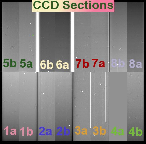
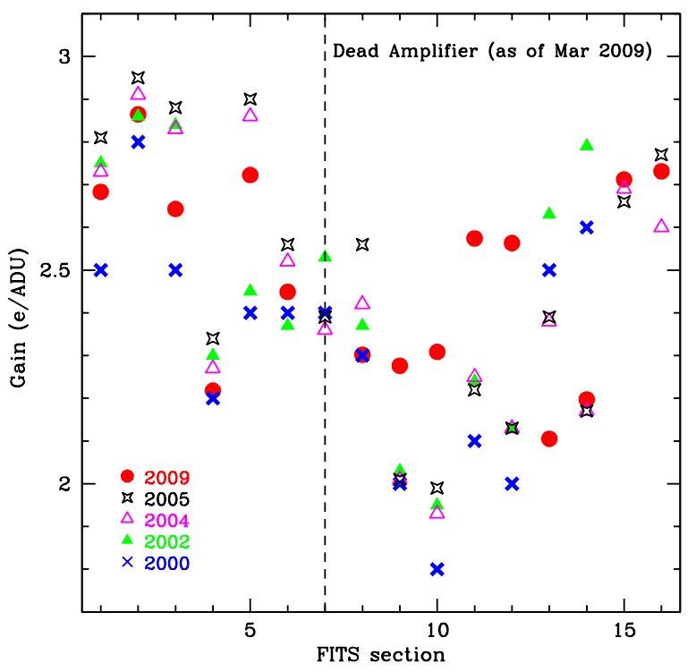
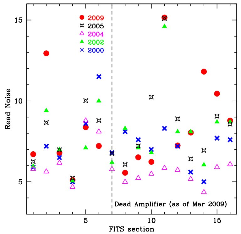
Last updated: K. Olsen 27 August 2003
| Chip 1 | Chip 2 | Chip 3 | Chip 4 | Chip 5 | Chip 6 | Chip 7 | Chip 8 | ||
| Zero Point |
U | 2.217 (0.007) | 2.220 (0.005) | 2.231 (0.005) | 2.254 (0.008) | 2.234 (0.010) | 2.215 (0.005) | 2.216 (0.005) | 2.227 (0.009) |
| B | -0.107 (0.008) | -0.120 (0.008) | -0.115 (0.008) | -0.111 (0.009) | -0.111 (0.008) | -0.101 (0.008) | -0.106 (0.008) | -0.104 (0.008) | |
| V | -0.448 (0.008) | -0.472 (0.004) | -0.472 (0.004) | -0.476 (0.011) | -0.475 (0.004) | -0.471 (0.006) | -0.472 (0.005) | -0.475 (0.007) | |
| R | -0.636 (0.004) | -0.633 (0.004) | -0.648 (0.004) | -0.632 (0.004) | -0.628 (0.004) | -0.616 (0.004) | -0.629 (0.005) | -0.624 (0.006) | |
| I | 0.089 (0.010) | 0.118 (0.008) | 0.076 (0.010) | 0.094 (0.008) | 0.094 (0.004) | 0.123 (0.007) | 0.113 (0.011) | 0.088 (0.010) | |
| Color Term |
U | 0.027 (0.019) | 0.028 (0.015) | 0.021 (0.015) | 0.018 (0.019) | -0.025 (0.024) | 0.019 (0.016) | 0.015 (0.016) | -0.002 (0.021) |
| B | -0.069 (0.010) | -0.062 (0.010) | -0.058 (0.010) | -0.055 (0.011) | -0.056 (0.010) | -0.079 (0.011) | -0.081 (0.010) | -0.068 (0.010) | |
| V | 0.038 (0.009) | 0.044 (0.005) | 0.042 (0.005) | 0.060 (0.012) | 0.063 (0.005) | 0.041 (0.007) | 0.039 (0.006) | 0.056 (0.008) | |
| R | -0.025 (0.008) | -0.037 (0.008) | -0.022 (0.008) | -0.032 (0.008) | -0.028 (0.008) | -0.045 (0.008) | -0.035 (0.010) | -0.029 (0.011) | |
| I | 0.009 (0.009) | -0.002 (0.007) | 0.008 (0.009) | 0.006 (0.007) | 0.003 (0.004) | -0.002 (0.006) | 0.003 (0.011) | 0.011 (0.010) |
The equations used to fit the standard star photometry are of the form:
u = U + A0 + A1X + A2(U-B)
b = B + B0 + B1X + B2(B-V)
v = V + C0 + C1X + C2(B-V)
r = R + D0 + D1X + D2(V-R)
i = I + E0 + E1X + E2(V-I)
where lowercase letters are the instrumental magnitudes (-2.5log(ADU sec-1)+25), X is the airmass, and capital letters are the standard magnitudes.
| Chip (1) | 1 | 2 | 3 | 4 | 5 | 6 | 7 | 8 |
| FITS section | 1 | 2 | 3 | 4 | 5 | 6 | 7 | 8 |
|
Gain (e-/ADU) 09 Nov 2009 (2) |
2.8 | 2.3 | 2.4 | 2.7 | 2.3 | 2.5 | 2.0 | 2.7 |
|
Read noise (e-) 09 Nov 2009 (3) |
14.7 | 5.7 | 6.3 | 5.2 | 8.6 | 13.5 | 6.9 | 12.3 |
|
Full well (e-) 31 Aug 2000 |
48,000 | 34,500 | 28,000 | 29,000 | 43,500 | 52,000 | 41,000 | 21,500 |
1. When looking at a Mosaic image, the 4 lower segments are denoted from left to right: 1, 2, 3, 4. Across the top, from left to right: 5, 6, 7, 8 (see plot below).
2. Gain measured from Transfer curve.
3. Read noise calculated from standard deviation of a bias frame × gain.
Back to Mosaic II [15]
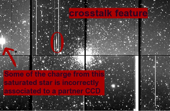
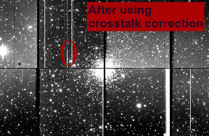
Crosstalk Correction Files
Crosstalk file for 8-channel mode [51], November 2010
Back To Mosaic II [40]
Updated: April 2010 by Andrea Kunder
The Mosaic 2 CCDs have relatively few bad pixels, mostly around the edges and in CCD #3.
Bad pixels do not respond to light at all, or respond in a nonlinear way. These can be removed from data using a bad pixel mask. The current bad pixel mask in the mscred package is from 2001, so we recommend using the updated bad pixel mask found here.
![]() [52]
[52]
 [53]
[53]
You can create your own bad pixel mask by taking appropriate flat field observations, or download the most recent mask image below.
Bad Pixel Mask for 8-channel mode [54], 14 May 2010
The bad pixel masks are not trimmed. Hence, your images must not be trimmed in order to use them.
Here are the steps to use the bad pixel masks:
hedit *.fits[1] BPM CAL0510/bpm1_0510.pl veri- show+
hedit *.fits[2] BPM CAL0510/bpm2_0510.pl veri- show+
hedit *.fits[3] BPM CAL0510/bpm3_0510.pl veri- show+
hedit *.fits[4] BPM CAL0510/bpm4_0510.pl veri- show+
hedit *.fits[5] BPM CAL0510/bpm5_0510.pl veri- show+
hedit *.fits[6] BPM CAL0510/bpm6_0510.pl veri- show+
hedit *.fits[7] BPM CAL0510/bpm7_0510.pl veri- show+
hedit *.fits[8] BPM CAL0510/bpm8_0510.pl veri- show+
| images | = | @objects.list | List of Mosaic CCD images to process |
| (output | = | ) | List of output processed images |
| (bpmasks | = | ) | List of output bad pixel masks |
| (ccdtype | = | object) | CCD image type to process |
| (noproc | = | no) | List processing steps only? |
| (xtalkco | = | yes) | Apply crosstalk correction? |
| (fixpix | = | yes) | Apply bad pixel mask correction? |
| (oversca | = | yes) | Apply overscan strip correction? |
| (trim | = | yes) | Trim the image? |
| (zerocor | = | yes) | Apply zero level correction? |
| (darkcor | = | no) | Apply dark count correction? |
| (flatcor | = | yes) | Apply flat field correction? |
| (sflatco | = | no) | Apply sky flat field correction? |
| (split | = | no) | Use split images during processing? |
| (merge | = | no) | Merge amplifiers from same CCD? |
| (xtalkfi | = | xtalk090401.txt) | Crosstalk file |
| (fixfile | = | BPM) | List of bad pixel masks |
| (saturat | = | ) | Saturated pixel threshold |
| (sgrow | = | 1) | Saturated pixel grow radius |
| (bleed | = | 20000.) | Bleed pixel threshold |
| (btrail | = | 15) | Bleed trail minimum |
| (bgrow | = | 1) | Bleed pixel grow radius |
| (biassec | = | !biassec) | Overscan strip image section |
| (trimsec | = | !trimsec) | Trim data section |
| (zero | = | Zero.fits) | List of zero level calibration images |
| (dark | = | ) | List of dark count calibration images |
| (flat | = | Dflat.fits) | List of flat field images |
| (sflat | = | Sflat.fits) | List of secondary flat field images |
| (minrepl | = | 1.) | Minimum flat field value |
| (interac | = | no) | Fit overscan interactively? |
| (functio | = | legendre) | Fitting function |
| (order | = | 1) | Number of polynomial terms or spline pieces |
| (sample | = | *) | Sample points to fit |
| (naverag | = | 1) | Number of sample points to combine |
| (niterat | = | 1) | Number of rejection iterations |
| (low_rej | = | 3.) | Low sigma rejection factor |
| (high_re | = | 3.) | High sigma rejection factor |
| (grow | = | 0.) | Rejection growing radius |
| (fd | = | ) | |
| (fd2 | = | ) | |
| (mode | = | ql) |
mscred> display DividedFlat.fits[1] 1 overlay=bpm1_0102.pl
Back To Mosaic II [15]
Updated: May 2010 by Andrea Kunder
THIS INSTRUMENT HAS BEEN RETIRED. INFORMATION PROVIDED HERE IS FOR REFERENCE ONLY
Here is a schematic layout of Mosaic 2:
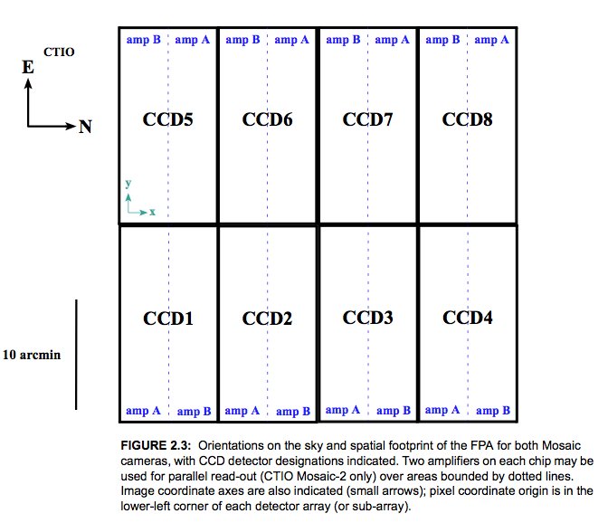
The CCD4, amplifier A died in 2009. Hence, nothing is read out from this part of CCD4. You have two options:
An example image is shown here (click to enlarge):
 [62]
[62]
* In 16 channel mode the read-out time is 100 s
The whole image will be usable as seen here:
 [63]
[63]
In 8 channel mode the read-out time is 150 s
Back To Mosaic II [15]
Page created: April 2010 by Andrea KunderEvery so often, something or other happens which causes the Arcon software to hang, or otherwise get confused. In the vast majority of cases this can be fixed by simply restarting the software running on ctioa0. This takes only a couple of minutes.
On ctioa0:
 [64]
[64]
 [65]
[65]
 [66]
[66]
Arcon crases can be avoided or ameliorated through the following practises:
Back To Mosaic II. [15]
Page created: 7 November 2006 by Tim Abbott
There are times when the TCS does not collect information about an image, and hence, your image headers may not have all required information. You can see if your headers have the required information by typing in the iraf terminal:
cl> hsel obj*fits[1] $I,RA,Dec,filter yes
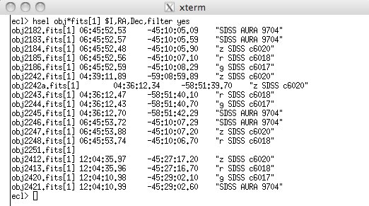
In this example, "obj2251.fits" does not have the RA, Dec, or filter in the header.
Before you do anything, make sure to save a copy of the original image.
You may use the iraf task "hedit" to update the parameters. Make sure to edit every single extension on your image.
You may download the task 'repairhdr' that will fix your headers as well. The advantage with downloading this tasks is that you only have to type one command, and then all 8- or 16-extensions will be updated.
repairhdr
The task "repairhdr" is a general task that can be used to fix any additional header information.
Download repairhdr here [68]
run the task
Place the task in a directory and make note of where you have saved it. (e.g.: /Users/mydownloads/)
Go to the directory that your images are in:
> cd /Users/myname/DATA/
Define the task:
> task repairhdr = /Users/mydownloads/repairhdr.cl
Call the task to update any fields:
> repairhdr obj2251.fits RA 06:45:53.74 ver-
> repairhdr obj2251.fits DEC -45:10:06.70 ver-
> repairhdr obj2251.fits filter "g SDSS c 6017" ver-
Back To Mosaic II [40]
Page created: February 2011 by Andrea Kunder
The original problem(s), described here [69], have been partially resolved. The residual errors in FITS keyword timing are not likely to present problems for the vast majority of observers, but some should still be aware of the following.
There are a number of FITS header keywords relevant to Mosaic exposure timing. Among them are:
The majority of other Mosaic header time values are derived from DATE-OBS by calculation.
In the absence of a known, precise time source with which to directly compare DATE-OBS and LSTHDR, we can only reliably report on the differences between the two. Previously [70], significant drifts and glitches between the two have been observed and have compromised some data. Since the Mosaic run of May 2003, the Arcons have been synchronising their clocks via NTP and time values are considerably better behaved.
Besides a fixed offset of a few seconds, local sidereal time as calculated from the DATE-OBS keyword matches that reported in the LSTHDR to within an envelope ~1.5 sec. wide. The variation of differences between the two clocks shows structure which suggests truncation error, or something like it, may be the cause.
LSTHDR is subject to occasional dropouts, possibly related to communications problems with the TCS, in which it is not available in the Mosaic FITS header.
Absolute timing values are not reliable in dark and focus frames.
The graph below shows the difference between LST as calculated from the DATE-OBS keyword and that reported in the LSTHDR keyword for 2003 up to September. The large deviations are all associated with dropouts in LSTHDR, sequences of darks and focus frames.
The graph below is the same as above, but expanded on the y axis. Note the significant improvement in bahaviour of the two clocks starting in May 2003. After this date, points more distant than ~1sec from a difference between the two clocks of ~4sec are associated with focus frames.
The plot below shows data from 3 nights in June 2003 on an expanded scale to show the behaviour in the course of a night. There is clearly some quantizing effect, but no longer any large-amplitude steady drifts.
back to Mosaic II [15]
There exist unresolved problems with the absolute timing of Mosaic exposures. For most programs, these are not likely to present serious problems but observers should be aware of the following.
There are a number of FITS header keywords relevant to Mosaic exposure timing. Among them are:
DATE-OBS - this is the UT time and date of the beginning of the exposure as derived from the Arcon detector controller. Arcon timing is derived from the host computer at boot time.
LSTHDR - this is the local sidereal time as acquired from the telescope control system at a time near to the beginning of the exposure. The telescope's LST is derived from a GPS system sited in the 1.5-m dome and is believed to be well-behaved.
The majority of other Mosaic header time values are derived from DATE-OBS by calculation.
The free-running Arcon clock appears to suffer from glitches and drifts:
The glitches result in discontinuous changes in the Arcon timing of amplitudes of several days. These tend to be obvious to the observer and will impact automated data reduction procedures which are sensitive to DATE-OBS. Their cause has not yet been identified.
Unfortunately, the Arcon internal clock is inadequate for precision timing on its own. Drifts of several seconds over the course of a night may be observed.
Arcon timing is reset at boot time, so drifts and glitches can be corrected by rebooting the system. It is advised that this be done at the beginning of each night anyway.
The offset between LSTHDR and DATE-OBS can be calibrated by an exposure taken immediately after a reboot. Compromised data can be repaired by back-calculating UT from LSTHDR and applying this offset.
This procedure should result in a precision of better than 1 sec.
The graph below shows the difference between DATE-OBS and the keyword WEATDATE. WEATDATE is derived from the weather station and provides an additional comparison, although it should not be used as any form of timing reference. The large excursions near October 2001 should be ignored, but the points around 3 days offset in 2002 illustrate the large timing glitches. (The offsets are all plotted as if positive, but many are negative.)
 [71]
[71]
The graph below shows the timing drifts as sideral seconds in the 2001 and 2002 calendar years.
 [72]
[72]
Finally, this chart shows a three week period with the offsets color-coded by type.
 [73]
[73]
A Note on focussing the Mosaic camera
(For basic instructions on measuring and setting focus go here [3].)
1. focus-by-eye with a large focus step value
2. Chris's roundest-image technique.
Do an "mscexam" and hit "m". If the resulting profile looks North-South elongated like this:
 [74]
[74]
then you must decrease the focus value.
3. Collecting lots of stars in a focus image with ~100 unit steps and aiming at the middle of the flattish/noisy portion of the through-focus FWHM curves.
Back To Mosaic II [15]
Page created: 23 March 2004 by Tim Abbott Updated: April 2010 by Andrea KunderMosaic temperature control: a warning. If you are using z' filter, read this!
In late 2003, it was discovered that the temperature control loop for the CCDs in the Mosaic camera is not closed. That is, the temperature of the focal plane is free to vary according to its instantaneous thermal load and coupling quality with the LN2 tank. A warning is sounded if this temperature moves more than ten degrees away from 165K, but otherwise, the temperature can vary by several degrees Celcius within a night and by as many as 10-12 degrees Celcius over the course of an observing block.
It is not clear how long this has been the case. Possibly (probably?) since the instrument was commissioned.
The consequence will be to produce QE variations at the red end of the spectrum. In particular data taken with the SDSS z' filter will be affected, as for any other filter where the red cutoff is set by the drop off of the CCD QE rather than the filter itself. The variation in QE of a silicon detector can show up to 1% variation per degree temperature change in the far red.
Created: 23 March 2004, by Tim Abbott
You need to do two things: (a) change the name of the file, and (b) change the information in the header describing the "image type".
The linearity should be good to <1% up to 20,000 and 40,000 adu, depending on which CCD. The point at which each amplifier saturates is posted on the main CTIO Mosaic web page. The amplifiers probably begin to go non-linear within 10% of these values. Note that there are SIGNIFICANT variations, so one must be careful when specifying the saturation value.
Before fixing any headers, save a copy of the original image.
| epar fixhdr1 | ||
| image = | obs1011.fits | Image to update header |
| ra = | 05:13:02.71 | right ascension |
| dec = | +09:51:05.00 | declination |
| filter = | V c6026 | filter |
| (epoch = | 2000.) | epoch of coordinates |
| (hdrpath = | home$uparm/) | Path to header files |
| (update = | yes) | update image headers |
| verbosi = | yes) | verbose mode |
| (mode = | q) |
The tasks to use are mscsplit and mscjoin.
Lindsey Davis described some of the details of the WCS calculations in this email about Mosaic WCS computations.
Frank Valdes described this correction in an email about using the task 'pixarea' in the mscred package.
Back To Mosaic II [40]
Last updated: April 2010 by AMK
To prepare the instrument, you need to run 'SetFiles' to configure all of the Arcon setup files. The Standard SetFiles [75] page shows a sample run of SetFiles for the standard 8 CCD mode of MosaicII.
Occasionally the user would prefer to use a single CCD instead of the whole Mosaic. This requires the support person to 'SetFiles' with slightly different answers. The Single controller SetFiles [76] page shows a sample run of SetFiles for this mode of MosaicII.
Do "epar engpars" and change parameter "amplifiers" to either "a1a2" (for a amplifiers), or "b1b2" (for b amplifiers), or "all" for all 16 amplifiers. As one of the a-amplifiers is not working, it is best to use "b1b2" for 8 channel mode. Then you must do "setdet f+", just go in and out of this, it will then recompile the waveforms suitably. Note that we are using the 16 channels or 8 "b" amplifiers as default.
NOTE: If you started up in 8 channel mode and are changing to 16 channel, you should do a "all video cal in" to recalibrate the electronics (specifically the 8 channels that weren't recalibrated when you started up in 8 channel mode. This should be typed in the Arcon console (arcon_user) box.
Check out Frank's email explaining the process [77].
For example, how does one move the data acquisition from ctioa0 to ctioa1? This detailed instruction list [78] will guide you through the process. It should only take about 15 minutes if both machines have Alta boards.
Using ~/scripts/pimfeed. First, on the data acquisition machine, in the blue IRAF (Data Acquisition) window, cd to where you want the images to go and take 1 exposure (for example, a test exposure). This sets the directory for the recovered files to go to. Then open a UNIX window (an xterm, for example), cd to the directory you chose above, and then do a ls -l /rawdat. Note the ID number of the files you want to recover (the number behind the "xpim", without the underscore. For example, if the ls resulted in something like...
mosaic@ctioa1>/rawdat% ls -al
total 102754
drwxrwxr-x 2 mosaic 512 Dec 13 06:31 .
drwxr-xr-x 8 root 512 Dec 9 10:06 ..
-rw-rw-r-- 1 mosaic 3024 Dec 13 05:00 fits18422.141
-rw-rw-r-- 1 mosaic 1707 Dec 13 05:01 hdr18422.141
-rw-rw-rw- 1 mosaic 32 Dec 13 05:01 xpim18422.141_0
-rw-rw-rw- 1 mosaic 35032680 Dec 13 05:04 xpim18422.141_1
-rw-rw-rw- 1 mosaic 35032680 Dec 13 05:04 xpim18422.141_2
-rw-rw-rw- 1 mosaic 35032680 Dec 13 05:04 xpim18422.141_3
... then you want to use the ID number 18422.141. So in the UNIX window, type~/scripts/pimfeed 18422.141. This should start the transfer of the image to ctio4m. Watch the DCA on ctio4m to see if things are working correctly.
If the Arcon windows ARE running, then in the IRAF Acquisition window, type
If the Arcon windows are NOT running, try...
Chris Smith
Occasionally, the Arcon controllers get into a weird state.
SOLUTION: There are roughly 4 levels of severity with which the user can respond:
The most common explanation for this is that msmid is not running on the data acquisition machine.
SOLUTION: start up msmid on the data acquisition machine. This is described in step 2 of the detailed instruction list [78] for changing data acquisition computers.
This usually happens because there is another copy of the GUI running on the data acquisition machine. The title of the GUI usually says "MCCD Configuration - Monitor mode".
SOLUTION: kill off all other 'arInt' processes. First do a ps aux | grep Int. Look for any 'arInt' processes. Kill these with kill -9 (process id number). Then you can EITHER restart Arcon (~3 minutes), OR, if you're in a hurry, you can go to the blue IRAF (Data Acquisition) window and type gwcclose, return, thengwcopen, and return. This should bring up both GUI windows.
try b1 vtt telemetry. The 'b1' can be replaced by b2, b3, and b4 to check communication and voltages on each box.
Try turning off triggering. To do this, in the blue IRAF (Data Acquisition) window, type engpars and change the trigger parameter to 'no'. Then run setdet to download this change to the controller. Each box will now run on its own, not waiting for the master for trigger signals.
To start direct communication with the MSE system (which is connected via the serial port on the data acquisition machine), do the following...
Occasionally, the one or both PVMs get into a weird state. This can be seen by typing "pvm", and then "conf" on either ctioa0 or ctioa8. Either machine should list both ctioa0 and ctioa8 as connected.
SOLUTION: Restart the PVMs from zero, following the instructions on the PVM restart [80] page.
Chris Smith
This is a brief introduction describing how we use VNC (Virtual Network Computing) [81] to display the various windows which control use of the NOAO Mosaic imager, specifically Mosaic II at CTIO. The advantage of this is that support staff (both on the mountain and downtown) can monitor the use of the instrument, actually SEEING in real time any errors that appear.
If the Mosaic has been up and running, the user should only have to click on the icons "Start_DCA", "Ximtool", and "Arcon". These buttons run the scriptsstart_dca_a8, start_disp_a8, and start_a0, which are found in the/ua80/mosaic/bin directory. The scripts start up the servers, if necessary, and then the VNC viewers.
These icons and/or scripts should bring up three VNC viewer windows (one for Arcon Acquisition, with a blue background, one for the DCA, with a green background, and one for the real-time display, also with a green background) on ctioa8. Once these come up, use the menus (right mouse button inside VNC window) to start up Arcon in the blue window, the DCA in the DCA window, and ximtool in the real-time display.
NOTE: The multiple Xview warnings which come up in the ARCON Acquisition window are harmless... we're just missing a font for the large countdown timer.
The following images show what should be the result of the instructions above. Click on either for a larger view.
 [82] [13] [14]
If pressing the icons produces no result, or the VNC clients start up but the menus appear inaccessible, you will probably have to kill the servers and restart them manually, as follows.
On ctioa8, open an xgterm or xterm window. All of the following commands below (where it says "type...") should be typed into this window.
1. rsh ctioa0 "source .login; vncserver -kill :9"
2. rsh ctioa0 "source .login; vncserver :9 -cc 3 -alwaysshared -geometry 1060x800"
This should start the vncserver on ctioa0 and output the following text:
New 'X' desktop is ctioa0:9
Starting applications specified in /arc/mosaic/.vnc/xstartup
Log file is /arc/mosaic/.vnc/ctioa0:9.log
If line 2 generates an error message about a file in /tmp, remove the file (rsh ctioa0 "rm /tmp/file_name") and try line 2 again.
Clicking the "Arcon" button should now bring up the Arcon VNC viewer. If you would rather start the viewer manually , too, then type
The VNC viewer window should come up, and something like the following output should show up in the xgterm where you typed vncviewer.
[1] ####
VNC server supports protocol version 3.3 (viewer 3.3)
VNC authentication succeeded
Desktop name "mosaic's X desktop (ctioa0:9)"
Connected to VNC server, using protocol version 3.3
VNC server default format:
8 bits per pixel.
Colour map (not true colour).
Using default colormap and translating from BGR233. Pixel format:
8 bits per pixel.
True colour: max red 7 green 7 blue 3, shift red 0 green 3 blue 6
Got 237 exact BGR233 colours out of 256
Using 1 existing shared colours
In this xgterm window, you can now hit ctrl-X and type "bg" to put the vncviewer in background.
1. vncserver -kill :9
2. vncserver :9 -cc 3 -alwaysshared -geometry 700x700
This should start the vncserver on ctioa8 and output the following text:
New 'X' desktop is ctioa8:9
Starting applications specified in /ua80/mosaic/.vnc/xstartup
Log file is /ua80/mosaic/.vnc/ctioa8:9.log
Again, if starting the server produces an error message refering to a file in /tmp, remove the appropriate file in /tmp and repeat step 2.
Clicking the Start_DCA button should now bring up the VNC viewer. If you would rather start the viewer manually, type
The VNC viewer window should come up, and something like the following output should show up in the xgterm where you typed vncviewer.
[1] ####
VNC server supports protocol version 3.3 (viewer 3.3)
VNC authentication succeeded
Desktop name "mosaic's X desktop (ctioa8:9)"
Connected to VNC server, using protocol version 3.3
VNC server default format:
8 bits per pixel.
Colour map (not true colour).
Using default colormap and translating from BGR233. Pixel format:
8 bits per pixel.
True colour: max red 7 green 7 blue 3, shift red 0 green 3 blue 6
Got 237 exact BGR233 colours out of 256
Using 1 existing shared colours
Same machine: preferring raw encoding
In this xgterm window, you can now hit ctrl-X and type "bg" to put the vncviewer in background.
1. vncserver -kill :8
2. vncserver :8 -cc 3 -alwaysshared -geometry 700x700
This should start the vncserver on ctioa0 and output the following text:
New 'X' desktop is ctioa8:8
Starting applications specified in /ua80/mosaic/.vnc/xstartup
Log file is /ua80/mosaic/.vnc/ctioa8:8.log
Again, if starting the server produces an error message, remove the appropriate file in /tmp and repeat step 2.
Clicking the Start_DCA button should now bring up the VNC viewer. If you would rather start the viewer manually, type
The VNC viewer window should come up, and something like the following output should show up in the xgterm where you typed vncviewer.
[1] ####
VNC server supports protocol version 3.3 (viewer 3.3)
VNC authentication succeeded
Desktop name "mosaic's X desktop (ctioa8:8)"
Connected to VNC server, using protocol version 3.3
VNC server default format:
8 bits per pixel.
Colour map (not true colour).
Using default colormap and translating from BGR233. Pixel format:
8 bits per pixel.
True colour: max red 7 green 7 blue 3, shift red 0 green 3 blue 6
Got 237 exact BGR233 colours out of 256
Using 1 existing shared colours
Same machine: preferring raw encoding
In this xgterm window, you can now hit ctrl-X and type "bg" to put the vncviewer in background.
Sometimes VNC doesn't gracefully let go of the X display it is using (sometimes for a few minutes, sometimes longer). If, for example, one of the VNC servers crashes (which I've never seen happen), and the user immediately tries to restart it, one may get an error saying that VNC is running on :9, even though it isn't. Such an error might look like
mosaic@ctioa8% startvnc_a0
A VNC server is already running as :9
[1] 3328
vncviewer: ConnectToTcpAddr: connect: Connection refused
Unable to connect to VNC server
[1] Exit 1 vncviewer ctioa0:9 -passwd /ua82/mosaic/.vnc/passwd
To get around this problem, first try waiting about 2-3 minutes before running startvnc again. This should be enough time to allow the socket to be released. If this fails, try going through the manual startup and substitute another number, for example 8, whereever you see 9 in the above manual example. This will start up the VNC sessions on X display :8, but otherwise should be the same.
IF ALL ELSE FAILS: You can bypass VNC completely and start up the windows directly. To do this...
This should bring up the normal Arcon windows directly on the ctioa8 display. To exit this Arcon session, go back to the xgterm with the ctioa0 prompt and type
This should kill all of the Arcon windows on ctioa8.
To connect from other machines, you must (of course) have the VNC viewer application installed. This should be installed on most workstations, and can be downloaded for PCs and Macs from the VNC Homepage [83].
To view a Mosaic session, simply use the VNC viewer application to connect to ctioa0:9 (for the data acquisition windows) or ctioa8:9 (for the DCA windows). You must know the password to enter. NOTE!! You should ALWAYS enter as VIEWONLY unless you are trying to remotely help the observer. If you do not know how to do this, DON'T CONNECT!
Please send comments and questions to: Chris Smith: csmithATctio.noao.edu Last updated: 29 November 2002 by Chris Smith
| Sacar tapa del corrector | Remove cover for ADC corrector |
| Hacer flip a Mosaico | Flip Mosaic |
| Cambiar llaves de llenado de nitrogeno | Change valve to fill the dewar |
| Revisar lista de filtros para instalacion | Check filter list, change if needed |
| Hacer balance | Balance telescope |
| Revisar/Alinear lamparas de calibracion | Check and align flat field lamps |
| Revisar tanque de nitrogeno para llenado | Check that nitrogen tank has liquid nitrogen in it |
| Poner protector de genero negro en chimenea | Put gage protector on chimney |
| Poner tapon de madera en boquilla de llenado | Put wooden plug to nozzle |
|
Revisar si ctioa0 "is up and running" ( PVM's and VNC 's) |
Check out ctioa0 |
|
Revisar si ctioa8 "is up and running" (PVM's and VNC's) |
Check out ctioa8 |
To check VNC's, the commands and results should look like the following...
mosaic@ctioa0% ps aux | grep vnc
| mosaic | 406 | 0.0 | 0.8 | 2244 | 2984 | ? | S | Apr 14 | 85:57 | Xvnc :9 -desktop X -http |
| mosaic | 408 | 0.0 | 0.0 | 36 | 0 | ? | IW | Apr 14 | 0:00 | /bin/sh /arc/mosaic/.vnc |
| mosaic | 11581 | 0.0 | 0.1 | 56 | 232 | pb | S | 11:33 | 0:00 | grep vnc |
mosaic@ctioa8% ps aux | grep vnc
| mosaic | 6281 | 0.0 | 0.1 | 4304 | 2720 | pts/0 | S | 10:49 | 0:01 | Xvnc :9 -desktop |
| mosaic | 6541 | 0.8 | 0.2 | 6124 | 4568 | pts/0 | S | 11:00 | 0:11 | Xvnc :8 -desktop |
| mosaic | 7465 | 0.0 | 0.0 | 1728 | 592 | pts/7 | S | 11:23 | 0:00 | grep vnc |
To check that PVM is working and correctly configured on both machines
mosaic@ctioa0% pvm
pvmd already running.
pvm> conf
2 hosts, 2 data formats
| HOST | DTID | ARCH | SPEED |
| ctioa0 | 40000 | SUN4 | 1000 |
| ctioa8 | c0000 | LINUX | 1000 |
pvm> quit
pvmd still running.
mosaic@ctioa8% pvm
pvmd already running.
pvm> conf
2 hosts, 2 data formats
| HOST | DTID | ARCH | SPEED |
| ctioa0 | 40000 | SUN4 | 1000 |
| ctioa8 | c0000 | LINUX | 1000 |
pvm> quit
pvmd still running.
If EITHER does not look like this, it is best to simply start from the beginning.
This involves killing the pvm processes on BOTH ctioa0 and ctioa8 and then
restarting them. To do this, follow the instructions on restarting the pvm [80].
| Partir la sesion de VNC ( vncviewer) de Arcon en ctioa0 | Start Arcon VNC session on ctioa0 |
| Partir la sesion de VNC ( vncviewer ) de DCA en ctioa8 | Start DCA VNC session on ctioa8 |
| Partir la sesion de VNC ( vncviewer ) de IRAF en ctioa8 | Start IRAF VNC on ctioa8 |
| Partir sesion de Arcon con "Restart Arcon" | Start Arcon session with "Restart Arcon" |
| Fijarse de que no haya errores en la partida de Arcon | Take a look at Arcon window for signs of problems |
| Fijarse de TCS y MSE | Check the TCS and MSE boxes in the Mosaic GUI. |
| Configurar la lectura de CCD ( 8 o 16 Amps ) | Configure Mosaic to 8 or 16 Amps |
| Tomar un "test" de bias y fijarse que termine bien | Take a test bias, and make sure it looks good |
| Crear directorio de observacion y directorio de pruebas | Create a directory for the observer and also for testing |
| En directorio de pruebas tomar secuencia de bias (20) | In the directory for testing, take a sequence of biases |
|
Tomar sequencia de "domeflats" en forma automatica ( "doobs") : 5 exp / filtro |
Take a series of dome flats 5 exposures/filter |
| Revisar que las cuentas de los bias son normales | Confirm bias counts are normal |
|
En directorio de pruebas revisar # de cuentas en "flats" de los filtros a usar |
Confirm counts listed on sign for given exposure time are approximately correct. |
| Revisar movimiento en rueda de filtros en ambas direcciones | Check filter wheel movement in both directions |
|
Revisar el listado de filtros con comando "wheel1" y si es necesario actualizar lista |
Check list of filters using "wheel1" command and make sure filters are appropriate for the nights run |
| Apagar bomba de vacio del secundario | Turn off vacuum pump for secondary mirror |
| Seleccionar instrumento en TCS | Select instrument in TCS |
| Mover switch selector de foco a PRIME | Move switch to prime focus |
| Chequear si los elementos del ADC estan trabajando | Check if ADC works |
| Chequear si las camaras de guiaje estan conectadas | Check that guider camera is connected |
| Revisar/inicializar el valor del foco en pedestal | Check and initialize value for pedestal focus |
Last updated June, 2010
This is a log of an actual run of SetFiles for MosaicII (SetFiles for MosaicI should be very similar). It demonstrates the setup for the standard 8 CCD Mosaic mode.
NOTE: the items in bold below are typed by the support person setting up the instrument. The (return) means simply hit the return key.
----------------------------------------------------------------------------------------------------------------------------------------------
ctioa1% SetFiles -a
/etc/Environment
File setup for those who like to answer LOTS of questions
+++ Getting current settings from /etc/Environment...
+++ Getting current settings from /etc/Init_CPU_Info.nex...
(?) Software version (/m2xp/arcon) : (return)
(?) Do you have a Mosaic (no) : yes
(?) Is this the Mosaic II (no) : yes
(?) Is controller #1 present (yes) : yes
(?) Is controller #2 present (no) : yes
(?) Is controller #3 present (no) : yes
(?) Is controller #4 present (no) : yes
(?) Is the CCD electronics available (yes) : (return)
(?) Select the bootable name. There are(is) 1 possible choice(s)
for this name, based on the information given before:
0 Select bootable that's not in the menu
1 ComSeq1234II.Ooo
selection (ComSeq1234II.Ooo -> 1) : (return)
ComSeq1234II
(?) Select the controller name. There are 21 possible
choices for this name:
0 Select controller not in the menu
1 Arcon2001
2 Arcon3001
3 Arcon3002
4 Arcon3003
5 Arcon3005
6 Arcon3006
7 Arcon3007
8 Arcon3008
9 Arcon3009
10 Arcon3010
11 Arcon3011
12 Arcon3012
13 Arcon3013
14 Arcon3014
15 Arcon3015
16 Arcon3016
17 Arcon3017
18 Arcon3018
19 Arcon3019
20 Arcon3020
21 Arcon3021
Enter controller #1, selection (Arcon3018 -> 18) : (return)
Enter controller #2, selection (Arcon3019 -> 19) : (return)
Enter controller #3, selection (Arcon3020 -> 20) : (return)
Enter controller #4, selection (Arcon3021 -> 21) : (return)
(?) Interface card:
0 None
1 Parsytec
2 Alta
selection (2) : (return)
(?) Link number used to download (0) : (return)
(?) Muxnex command line options (-m) : (return)
(?) Observatory name (CTIO) : (return)
(?) Telescope name:
0 Select telescope not in the menu
1 none
2 ct4m
3 ct60
4 ct1m
5 ct36
6 ctschmidt
7 kp4m
8 kp36
selection (ct4m -> 2) : (return)
(?) Focal station:
0 Select focal station not in the menu
1 none
2 cf
3 nf
4 pf
5 cf14
6 cf75
7 cf135
selection (pf -> 4) : (return)
(?) Instrument name:
0 Select instrument not in the menu
1 none
2 argus
3 bme
4 cfccd
5 cs4m
6 cs60
7 csccd
8 cspol
9 echccd
10 fpccd
11 nfccd
12 pfccd
13 mosaic
selection (mosaic -> 13) : (return)
++++++++++++++++++++ New Settings ++++++++++++++++++++
| Software root directory | /m2xp/arcon |
| Interface card | 2 (Alta) |
| RTD memory | 256 (8 Mbytes) |
| Link used to download | 0 |
| Muxnex command line options | -m |
| Bootable name | ComSeq1234II.Ooo |
| Hardware configuration | ComSeq1234II |
| Observatory name | CTIO |
| Telescope name | ct4m |
| Number of controllers | 4 |
| Controller name for Nexus#1 | Arcon3010 (SITe4096) |
| Controller name for Nexus#2 | Arcon3011 (unknown) |
| Controller name for Nexus#3 | Arcon3018 (unknown) |
| Controller name for Nexus#4 | Arcon3019 (unknown) |
| Instrument | mosaic |
| Focal station | pf |
NOTE: If you didn't get the questions to change the settings you
wanted to, then try 'SetFiles -help' to find the command line
option that best matches your needs.
(?) Do you want to install the changes (yes) : (return)
Installing files...
The old copy of /etc/Environment was saved as /etc/Environment.BAK
The old copy of /etc/Init_CPU_Info.nex was saved as /etc/Init_CPU_Info.nex.BAK
-------------------------------------------------------------------------------------------------------------------------------------------
The support person should then start up Arcon ('(Re)start Arcon' in OpenWindows menu) and check to that the system boots. It is probably best to answer "no" to the "synchronize parameters?" query during this startup. This allows for changes to be made in the parameters (such as detpars) before sending parameters out to the instrument and detectors.
It is usually recommended to do an 'End Arcon Session' after completing the setup, and then a '(Re)start Arcon', answering 'yes' to the "synchronize parameters?" query this time. This is not absolutely necessary, but it does confirm that the system will restart for the user when he/she does a '(Re)start Arcon' later.
This is a log of an actual run of SetFiles for MosaicII for the special case where the user only wants to use 1 or 2 CCDs of the array. This is CURRENTLY (Dec 99) configured to use Box #1, disabling CCD#1 and enabling only CCD#2 for use. CCD #1 is disabled to prevent crosstalk problems from showing up in CCD#2.
NOTE: the items in bold below are typed by the support person setting up the instrument. The (return) means simply hit the return key.
---------------------------------------------------------------------------------------------------------------------------------
ctioa1% SetFiles -a
/etc/Environment
File setup for those who like to answer LOTS of questions
+++ Getting current settings from /etc/Environment...
+++ Getting current settings from /etc/Init_CPU_Info.nex...
(?) Software version (/m2xp/arcon) : (return)
(?) Do you have a Mosaic (no) : yes
(?) Is this the Mosaic II (no) : yes
(?) Is controller #1 present (yes) : yes
(?) Is controller #2 present (yes) : no
(?) Is controller #3 present (yes) : no
(?) Is controller #4 present (yes) : no
(?) Is the CCD electronics available (yes) : (return)
(?) Select the bootable name. There are(is) 1 possible choice(s)
for this name, based on the information given before:
0 Select bootable that's not in the menu
1 ComSeq1234II.Ooo
selection (ComSeq1II.Ooo -> 1) : (return)
ComSeq1II
(?) Select the controller name. There are 21 possible
choices for this name:
0 Select controller not in the menu
1 Arcon2001
2 Arcon3001
3 Arcon3002
4 Arcon3003
5 Arcon3005
6 Arcon3006
7 Arcon3007
8 Arcon3008
9 Arcon3009
10 Arcon3010
11 Arcon3011
12 Arcon3012
13 Arcon3013
14 Arcon3014
15 Arcon3015
16 Arcon3016
17 Arcon3017
18 Arcon3018
19 Arcon3019
20 Arcon3020
21 Arcon3021
Enter controller #1, selection (Arcon3018 -> 18) : (return)
(?) Interface card:
0 None
1 Parsytec
2 Alta
selection (2) : (return)
(?) Link number used to download (0) : (return)
(?) Muxnex command line options (-m) : (return)
(?) Observatory name (CTIO) : (return)
(?) Telescope name:
0 Select telescope not in the menu
1 none
2 ct4m
3 ct60
4 ct1m
5 ct36
6 ctschmidt
7 kp4m
8 kp36
selection (ct4m -> 2) : (return)
(?) Focal station:
0 Select focal station not in the menu
1 none
2 cf
3 nf
4 pf
5 cf14
6 cf75
7 cf135
selection (pf -> 4) : (return)
(?) Instrument name:
0 Select instrument not in the menu
1 none
2 argus
3 bme
4 cfccd
5 cs4m
6 cs60
7 csccd
8 cspol
9 echccd
10 fpccd
11 nfccd
12 pfccd
13 mosaic
selection (mosaic -> 13) : (return)
++++++++++++++++++++ New Settings ++++++++++++++++++++
| Software root directory | /m2xp/arcon |
| Interface card | 2 (Alta) |
| RTD memory | 256 (8 Mbytes) |
| Link used to download | 0 |
| Muxnex command line options | -m |
| Bootable name | ComSeq1II.Ooo |
| Hardware configuration | optical |
| Observatory name | CTIO |
| Telescope name | ct4m |
| Number of controllers | 1 |
| Controller name for Nexus#1 | Arcon3018 (SITe4096) |
| Instrument | mosaic |
| Focal station | pf |
NOTE: If you didn't get the questions to change the settings you
wanted to, then try 'SetFiles -help' to find the command line
option that best matches your needs.
(?) Do you want to install the changes (yes) : (return)
Installing files...
The old copy of /etc/Environment was saved as /etc/Environment.BAK
The old copy of /etc/Init_CPU_Info.nex was saved as
/etc/Init_CPU_Info.nex.BAK
---------------------------------------------------------------------------------------------------------------------------------
The support person should then start up Arcon ('(Re)start Arcon' in OpenWindows menu) and check to that the system boots. It is probably best to answer "no" to the "synchronize parameters?" query during this startup. This allows for changes to be made in the parameters (such as detpars) before sending parameters out to the instrument and detectors. At this point one should run newpset all to reset parameters for the new setup. Then, if the user wants a 2048x2048 CCD (for example), one would run setdet and set
It is usually recommended to do an 'End Arcon Session' after completing the setup, and then a '(Re)start Arcon', answering 'yes' to the "synchronize parameters?" query this time. This is not absolutely necessary, but it does confirm that the system will restart for the user when he/she does a '(Re)start Arcon' later.
Subject: Creating and Installing OTF Flat Fields
Date: Fri, 25 Aug 2000 10:23:26 -0700 (MST)
From: Frank Valdes
To: mosaic-ccdATtucana.tuc.noao.edu, pmasseyATtucana.tuc.noao.edu
In response to a question from Phil I am posting an updated version of something I sent around last fall.
I post this here for anyone interested or who might need to create the OTF flats, and as a record of the process as currently performed. This was updated from the previous version dated "Oct 28, 1999" to include information about how to set things up for personal use during an observing run. The only problem is how observers can install the files for general
use. Right now the files are put in a system directory owned by IRAF. I am considering making the directories have world permissions but with all previously installed directories being protected.
This information will be available on-line with "help mscotfflat" after the next update of MSCRED.
Frank
1. Take one or more flat fields. The count levels have to be below 30000. If not divide the values by a number either before or after processing using MSCARITH. Since the OTF flats are spatially binned and digitized to reduce size it probably is not very useful to create a high quality flat from multiple exposures, a single exposure should be fine.
2. Process the flat(s). The processing should be only overscan and trim. If combining multiple flats with FLATCOMBINE set the processing as noted. The processing should save the raw exposures in the Raw subdirectory (or whatever is set for the "backup" parameter in MSCRED).
3. Run MSCOTFFLAT with the default values. The output name must be one word (that is an acceptible directory name) and should be the standard identifier for the filter. Typically this would be the first word of the filter name recorded in the header (with any characters which are not letters, numbers, or '.' replaced with '_'). The template name is one of the raw exposures.
ms> mscotfflat flat001 B Raw/flat001
This will create a subdirectory, B in this example, with the number of pl files equal to the number of extensions.
3a. You can check if things make sense by the size of the pl files being approximately 0.6-1.6Mb. You can also display the files and compare with the original data using:
ms> display B/flat1 1 fill+ ...
ms> display flat00[1] 2 fill+ ...
They should be very similar to the flat from which they were derived.
4. To use during your run with the real-time DCA display you would set the calibration directory in the DCA GUI to point to the parent directory containing the subdirectories of pl files (the directory you were in when you ran MSCOTFFLAT). This is done from the "Edit" menu, selecting "Path Params", editing the "Calibration Dir" field, and finally clicking "Apply". Also if you are going to use MSCDISPLAY with "process=yes" then go to the "mimpars" parameters and set the "caldir" directory parameter there too. Remember that directories in IRAF must end with '/' (or '$' for logical directories).
If you do nothing else the software will look in the specified calibration directory for a subdirectory which matches the first word of the filter string in the image header (with any characters that are not letters, numbers, or '.' changed to '_'). If you want to translate the header filter name to some other (directory) name you can add a "cal.men" file where the first column is the filter name (quoted if there are blanks) and the second column is the directory name. This file is also used to set the override choices for the filter in the DCA GUI.
The following is done to install the OTF directory for general use and requires the IRAF login.
5. Login as IRAF and go to the standard calibration directory:
| /iraf/extern/mscdb/noao/ctio/4meter/caldir/Mosaic2A | # CTIO 4m (8 A amps) |
| /iraf/extern/mscdb/noao/ctio/4meter/caldir/Mosaic2B | # CTIO 4m (8 B amps) |
| /iraf/extern/mscdb/noao/ctio/4meter/caldir/Mosaic2 | # CTIO 4m (16 amps) |
| /iraf/extern/mscdb/noao/kpno/4meter/caldir | # KPNO 4m |
| /iraf/extern/mscdb/noao/kpno/36inch/caldir | # KPNO 36inch |
| /iraf/extern/mscdb/noao/kpno/wiyn/caldir | # KPNO WIYN |
Transfer the OTF directory to that calibration directory. One way is
% (cd /md1/4meter/nite1; wtar B) | rtar -xv
6. Edit the cal.men file. The first column is the filter name as given in the data files under the FILTER keyword. The second name is the directory name. The order of the entries in the order in which the filters will appear in the DCA list. Note the DCA list is only used to override the automatic filter selection based on the filter keyword.
7. Remove the OTF directory in your data area. One way is with "!rm -rf
". You can also restore the original raw flats for taping by moving the files from the Raw subdirectory back to the data directory.
8. I am maintaining a master MSCDB directory that includes current OTF flats. This serves the purpose of a backup, the source to generate installation files, and the source to generate distribution files for users who might want them. So if you create OTF files please notify me.
See also
ms> phelp mscotfflat
Switching which computer acts as Mosaic data acquisition machine is fairly easy and fairly quick (15 min), if you know how to do it. Here is a detailed, straightforward example of how to do it. For this example, we show the move from ctioa0 to ctioa1.
1. move serial connection from ctioa0 to ctioa1
2. change nexus connections from ctioa0 to ctioa1 (4 cables "rj-11"), installing them in the same order.
IF ctioa1 has been running normal arcon, you also need to run SetFiles [75] to finish the setup, setting "Software version" to /m2xp/arcon.
Last updated: December 27, 1999 Please send comments to:
The main thing to check on regarding the PVMs is if they are connected to the proper machines. To check the status of the PVMs running on ctioa0 and ctioa8, open an xterm or xgterm and type:
mosaic@ctioa8% pvm
pvm> conf
2 hosts, 2 data formats
| HOST | DTID | ARCH | SPEED |
| ctioa0 | 40000 | SUN4 | 1000 |
| ctioa8 | c0000 | LINUX | 1000 |
pvm> quit
pvmd still running.
Here we see that the pvm on ctioa8 is running and connected to ctioa0 and ctioa8. If both of these don't show up, move to "Restarting the Mosaic PVMs" below. A similar output should be obtained on ctioa0 if all is well.
If the pvm on EITHER ctioa0 or ctioa8 is misconfigured or otherwise having problems, it is best to kill them and restart them. To do this first you must stop all pvms which are currently running. Then start them from ctioa0 (not ctioa8).
FIRST on ctioa8, type (in an xgterm)
mosaic@ctioa8% pvm
pvmd already running.
pvm> halt
mosaic@ctioa8%
Often on ctioa8 this will NOT stop the PVM. So you must check to see if it really stopped by typing
mosaic@ctioa8% ps aux | grep pvm
If there are any pvm processes still running, kill them by typing
mosaic@ctioa8% kill -9 procid
where procid is the process ID of the pvm process.
Finally (for ctioa8), check to see that there are no pvm files left in /tmp by typing
mosaic@ctioa8% rm /tmp/pvm*
THEN do the same steps above for ctioa0. The halt command in pvm usually works on ctioa0, but it is still good to make sure with the ps command.
To start the pvms up, open an xterm or xgterm on ctioa0 and type...
mosaic@ctioa8% pvm
pvm> conf
| HOST | DTID | ARCH | SPEED |
| ctioa0 | 40000 | SUN4 | 1000 |
pvm> add ctioa8
pvm> conf
2 hosts, 2 data formats
| HOST | DTID | ARCH | SPEED |
| ctioa0 | 40000 | SUN4 | 1000 |
| ctioa8 | c0000 | LINUX | 1000 |
pvm> quit
pvmd still running.
The pvm command starts up pvm on ctioa0, and the "add ctioa8" command starts the pvm up remotely on ctioa8. The "conf" command confirms that the pvm was started on ctioa8 and that the link between ctioa0 and ctioa8 has been established.
To confirm that all is running well, go to ctioa8 and type (in an xgterm)
mosaic@ctioa8% pvm
pvmd already running.
pvm> conf
2 hosts, 2 data formats
| HOST | DTID | ARCH | SPEED |
| ctioa0 | 40000 | SUN4 | 1000 |
| ctioa8 | c0000 | LINUX | 1000 |
pvm> quit
pvmd still running.
Last updated Nov 29, 2002 @ 12:30 AM by CSmith
(1) check that VNC is running on both ctioa0 and ctioa8 (no need to restart them if they are already running). The commands and results should look like the following...
- ON ctioa0
mosaic@ctioa0% ps aux | grep vnc
| mosaic | 406 | 0.0 | 0.8 | 2244 | 2984 | ? | S | Apr 14 | 85:57 | Xvnc :9 -desktop X -http |
| mosaic | 408 | 0.0 | 0.0 | 36 | 0 | ? | IW | Apr 14 | 0:00 | /bin/sh /arc/mosaic/.vnc |
| mosaic | 11581 | 0.0 | 0.1 | 56 | 232 | pb | S | 11:33 | 0:00 | grep vnc |
- ON ctioa8
mosaic@ctioa8% ps aux | grep vnc
| mosaic | 6281 | 0.0 | 0.1 | 4304 | 2720 | pts/0 | S | 10:49 | 0:01 | Xvnc :9 -desktop |
| mosaic | 6541 | 0.0 | 0.2 | 6124 | 4568 | pts/0 | S | 11:00 | 0:11 | Xvnc :8 -desktop |
| mosaic | 7465 | 0.0 | 0.0 | 1728 | 592 | pts/7 | S | 11:23 | 0:00 | grep vnc |
(2) check that pvm is working and correctly configured on both machines
- ON ctioa0
mosaic@ctioa0% pvm
pvmd already running.
pvm> conf
2 hosts, 2 data formats @@
| HOST | DTID | ARCH | SPEED |
| ctioa0 | 40000 | SUN4 | 1000 |
| ctioa8 | c0000 | LINUX | 1000 |
pvm> quit
pvmd still running.
- ON ctioa8
mosaic@ctioa8% pvm
pvmd already running.
pvm> conf
2 hosts, 2 data formats
| HOST | DTID | ARCH | SPEED |
| ctioa0 | 40000 | SUN4 | 1000 |
| ctioa8 | c0000 | LINUX | 1000 |
pvm> quit
pvmd still running.
If EITHER does not look like this, it is best to simply start from the beginning. This involves killing the pvm processes on BOTH ctioa0 and ctioa8 and then restarting them. To do this, follow the instructions on restarting the pvm. [84]
Start up Arcon on ctioa0 and watch for errors in the Arcon Console window.
Also check the TCS and MSE boxes in the Mosaic GUI.
Confirm that counts listed on web page for given exposure times are approximately correct.
Last updated May 5, 2002
in Spanish
Al entrar a Mosaic
Los problemas comienzan aquí, ya que automáticamente debería abrir las ventanas de ctioa0 y DCA. Cuando el VNCserver fue terminado apropiadamente se puede abrir el VNCviewer a ctioa0 y DCA, directamente desde los íconos. En caso contrario, la ventana del DCA puede abrirse, pero no es posible seleccionar la partida del programa con el botón derecho y requiere hacer vncserver -kill ctioa8:9 y vncserver -kill ctioa8:8. Luego si esto ha sido solucionado, y ambos servidores ( ctioa8, ctioa0 ) estan en el listado de pvm ("conf" para listar; por ejemplo "add ctioa8" si ctioa8 no aparece; "quit" para salir), DCA partirá bien en caso contrario se deben agregar en el pvm. También pude ocurrir que haya otra sesión de DCA corriendo en cuyo caso, hay que verificar el PID con ps -Al | grep dca, y luego terminar el proceso con kill -HUP PID.
Verificar que se abre la ventana azul de Arcon y comienza el proceso de booteo. Durante este proceso debe abrirse la ventana de la GUI para shutter y filtros. En el momento que aparece, la etiqueta MSE debe aparecer en verde y mostrar las temperaturas del CCD. Si esto no sucede hay que matar la ventana dando ungwcclose desde la ventana de Arcon Acquisition, y luego desde una ventana del ctioa8 matar el proceso msmid determinado su PID con ps -ax | grep msmid y luego kill -9 PID. Después verificar que en el directorio /home/logs no está el archivo mseCommPortIsInUse! , si existiera borrarlo con un rm mseCommPortIsInUse!. A continuación hacer un start-msmid, en este punto co es obligatorio pero la mayoría de las veces requiere apagar la unidad de filtros en el pedestal, mediante el control remoto del power, en la sala de computadores. Finalmente desde la ventana Arcon Adquisition dar el comando gwcopen y la GUI debe abrirse funcionando normalmente.
Al salir de Mosaic
That's all folks.
Enrique & Manuel
Dark 600 sec, all amps
 [85]
[85]
Dark 600 sec B amps
 [86]
[86]
Links
[1] http://adsabs.harvard.edu/abs/2008SPIE.7014E..13D
[2] http://www.ctio.noao.edu/noao/content/mosaic-filters
[3] http://www.ctio.noao.edu/noao/content/cookbook
[4] http://www.ctio.noao.edu/noao/content/mosaic-manual
[5] http://www.noao.edu/kpno/mosaic/mosaic.html
[6] http://www.ctio.noao.edu/noao/content/faq
[7] http://www.ctio.noao.edu/noao/content/mosocs
[8] http://www.noao.edu/gateway/ccdtime/
[9] http://www.ctio.noao.edu/noao/content/adc
[10] http://www.ctio.noao.edu/new/Tools/Forms/EON/Form.php?telescope=Blanco%204-m
[11] http://www.ctio.noao.edu/new/Tools/Forms/EOR/Form.php?telescope=Blanco%204-m
[12] http://www.ctio.noao.edu/noao/content/Support-Notes
[13] http://www.ctio.noao.edu/noao/sites/default/files/instruments/imagers/vnca8dca.jpg
[14] http://www.ctio.noao.edu/noao/sites/default/files/instruments/imagers/vnca8xim.jpg
[15] http://www.ctio.noao.edu/noao/content/mosaic-ii-ccd-imager
[16] http://www.ctio.noao.edu/noao/content/mosaic-ii-ccds
[17] http://www.ctio.noao.edu/noao/content/previous-ccd-test-data-16-channel-mode
[18] http://www.ctio.noao.edu/noao/content/previous-ccd-test-data-8-channel-mode
[19] http://www.ctio.noao.edu/noao/sites/default/files/instruments/imagers/Mosaic_II_WCS_1999-2000.zip
[20] http://www.ctio.noao.edu/noao/content/4-m-MOSAIC-II-First-Pictures
[21] http://www.ctio.noao.edu/new/Telescopes/Blanco4m/TapeDrives.php
[22] http://www.ctio.noao.edu/noao/sites/default/files/instruments/imagers/m8vn.gif
[23] http://www.ctio.noao.edu/noao/sites/default/files/instruments/imagers/m16han.gif
[24] http://www.ctio.noao.edu/noao/sites/default/files/instruments/imagers/m16halong.gif
[25] http://www.ctio.noao.edu/noao/sites/default/files/instruments/imagers/baade.gif
[26] http://www.ctio.noao.edu/noao/sites/default/files/instruments/imagers/n6822v.jpg
[27] http://www.ctio.noao.edu/noao/sites/default/files/instruments/imagers/2002-05-17-report.txt
[28] http://www.noao.edu/kpno/manuals/dim/
[29] http://www.noao.edu/noao/meetings/spie98/mdhs.ps
[30] http://www.noao.edu/noao/meetings/spie98/wolfe.html
[31] http://www.noao.edu/noao/meetings/spie98/muller.ps
[32] http://www.ctio.noao.edu/instruments/arcon/arcon.html
[33] http://www.ctio.noao.edu/noao/content/ctio-575x575-inch-filters
[34] http://www.noao.edu/kpno/mosaic/filters/filters.html
[35] http://www.ctio.noao.edu/noao/content/pc-guider-documentation-v-32
[36] http://www.ctio.noao.edu/noao/sites/default/files/telescopes/pfadc_paper.ps
[37] http://www.ctio.noao.edu/noao/sites/default/files/telescopes/pfadc.gif
[38] http://iraf.noao.edu/projects/ccdmosaic/Reductions
[39] http://iraf.noao.edu/scripts/irafhelp?mscguide
[40] http://www.ctio.noao.edu/noao/content/MOSAIC-II-CCD-Imager
[41] http://www.ctio.noao.edu/noao/content/ccd-test-data-16-channel-mode
[42] http://www.ctio.noao.edu/noao/content/photometric-zero-points-color-terms
[43] http://www.ctio.noao.edu/noao/content/sky-rates
[44] http://www.ctio.noao.edu/noao/sites/default/files/instruments/imagers/bpm.tgz
[45] http://www.ctio.noao.edu/noao/sites/default/files/instruments/imagers/msccals.tgz
[46] http://www.ctio.noao.edu/noao/content/ccd-test-data-8-channel-mode
[47] http://www.ctio.noao.edu/noao/content/crosstalk-ctio-blanco-4m
[48] http://www.ctio.noao.edu/noao/sites/default/files/instruments/imagers/wcs8.db
[49] http://www.ctio.noao.edu/noao/content/bad-pixel-mask-8-channel-mode
[50] http://www.ctio.noao.edu/noao/content/historic-information-mosaic
[51] http://www.ctio.noao.edu/noao/sites/default/files/instruments/imagers/xtalk110510.txt
[52] http://www.ctio.noao.edu/noao/sites/default/files/instruments/imagers/badpixel1.jpg
[53] http://www.ctio.noao.edu/noao/sites/default/files/instruments/imagers/bpm_mask1.jpg
[54] http://www.ctio.noao.edu/noao/sites/default/files/instruments/imagers/BPM0610_8ch.tar
[55] http://www.ctio.noao.edu/noao/content/Amplifier-failure
[56] http://www.ctio.noao.edu/noao/content/amplifier-failure
[57] http://www.ctio.noao.edu/noao/content/arcon-crushes
[58] http://www.ctio.noao.edu/noao/content/fix-headers
[59] http://www.ctio.noao.edu/noao/content/limitations-absolute-timing
[60] http://www.ctio.noao.edu/noao/content/focusing
[61] http://www.ctio.noao.edu/noao/content/temperature-control
[62] http://www.ctio.noao.edu/noao/sites/default/files/instruments/imagers/ngc2808_16.jpg
[63] http://www.ctio.noao.edu/noao/sites/default/files/instruments/imagers/ngc2808.jpg
[64] http://www.ctio.noao.edu/noao/sites/default/files/instruments/imagers/crash.jpg
[65] http://www.ctio.noao.edu/noao/sites/default/files/instruments/imagers/crash7.jpg
[66] http://www.ctio.noao.edu/noao/sites/default/files/instruments/imagers/crash8.jpg
[67] http://www.ctio.noao.edu/noao/content/MOSOCS
[68] http://www.ctio.noao.edu/noao/sites/default/files/instruments/imagers/repairhdr.cl
[69] http://www.ctio.noao.edu/noao/content/Limitations-absolute-timing
[70] http://www.ctio.noao.edu/noao/content/Problems-Absolute-timing
[71] http://www.ctio.noao.edu/noao/sites/default/files/instruments/imagers/timing3.gif
[72] http://www.ctio.noao.edu/noao/sites/default/files/instruments/imagers/timing1.gif
[73] http://www.ctio.noao.edu/noao/sites/default/files/instruments/imagers/timing2.gif
[74] http://www.ctio.noao.edu/noao/sites/default/files/instruments/imagers/focus1.jpg
[75] http://www.ctio.noao.edu/noao/content/standard-setfiles-mosaicii-8-ccd-mode
[76] http://www.ctio.noao.edu/noao/content/single-controller-setfile-mosaicii-1-2-ccd-mode
[77] http://www.ctio.noao.edu/noao/content/how-make-otfs
[78] http://www.ctio.noao.edu/noao/content/changing-mosaic-data-acquisition-machines
[79] http://www.ctio.noao.edu/noao/content/using-vnc-mosaic
[80] http://www.ctio.noao.edu/noao/content/checking-and-restarting-mosaic-pvms
[81] http://en.wikipedia.org/wiki/Virtual_Network_Computing
[82] http://www.ctio.noao.edu/noao/sites/default/files/instruments/imagers/vnca0.jpg
[83] http://www.realvnc.com/
[84] http://www.ctio.noao.edu/noao/content/Checking-and-Restarting-Mosaic-PVMs
[85] http://www.ctio.noao.edu/noao/sites/default/files/instruments/imagers/dark600.gif
[86] http://www.ctio.noao.edu/noao/sites/default/files/instruments/imagers/dark600-b.gif