
At least read this!
Figure 1: Two views of the SOI mounted at one of the bent Cassegrain foci of the SOAR telescope. The smaller blue cylinder is the CCD mosaic dewar and is flanked by the two rectangular Leach controllers, the round black part is the cable wrap, and the large blue tube bolted onto the telescope is the main body of the instrument holding the linear ADC prisms, one of which can move over a distance of nearly one meter. The drawing shows the basic lay-out of the instrument in a cut-out view. From left to right the light encounters: ADC prisms, optics module, two filter slides, the shutter, and finally the CCD mosaic.
The SOI step-by-step Observer's Guide (NEW!) [30]
Optics:
The SOI optics consist of a 6 element focal reducer and field corrector, that converts the f/16.63 beam of the SOAR Telescope to f/9.82, preceeded by a linear, "trombone style", Atmospheric Dispersion Corrector (ADC). These optics were designed to deliver images of < 0.18 arcsec FWHM (equivalent to 80% encircled energy within D80 < 0.27 arcsec) at the zenith and <0.34 arcsec FWHM (D80 < 0.51 arcsec) at 70deg zenith distance, in each of the U, B, V, R, I broad band filters, and over the entire field. The glasses selected, and the use of SOLGEL over MgF2 coatings on all external surfaces ensure high transmission over the entire 310nm-1050nm passband. The measured transmission curve is shown below in Figure 2. Note that the transmission below 400nm is an underestimate of the true transmission due to limitations of the measuring device, and should be considered a lower limit.
Filters:
Filters are mounted in two filter cartrides each with space for 4 filters, plus one blank position, so that up to 8 filters can be installed in the instrument at any time. Although the cartridges were designed to be easily removeable, the process of changing them out still requires at least 30 minutes, and we currently have no spare cartridges. Thus it is strongly recommened that users design their programs to avoid filter changes during the night. Filters may be up to 100mm square and up to 10mm thick. Smaller filters may be accommodated with special adapters but must be at least 64mm square to avoid vignetting. To see the list of the currently available filters, together with transmission curves, click HERE [31]. Filters from the CTIO filter list [32] are also available.
CCDs:
The SOI focal plane is imaged onto a mini-mosaic of two CCD's with the following properties:
CCD mounting gap:
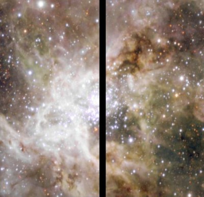
The two CCDs in the SOI are mounted with their long sides parallel and spaced 102 pixels apart, resulting in a 7.8" gap between the individual CCD images. This image of 30 Doradus shows how a single SOI image looks. The gap can be filled by taking dithered images. We recommend taking at least 3 images with 10" steps to produce a complete combined image with no gap.
Flat Fields and Fringing:
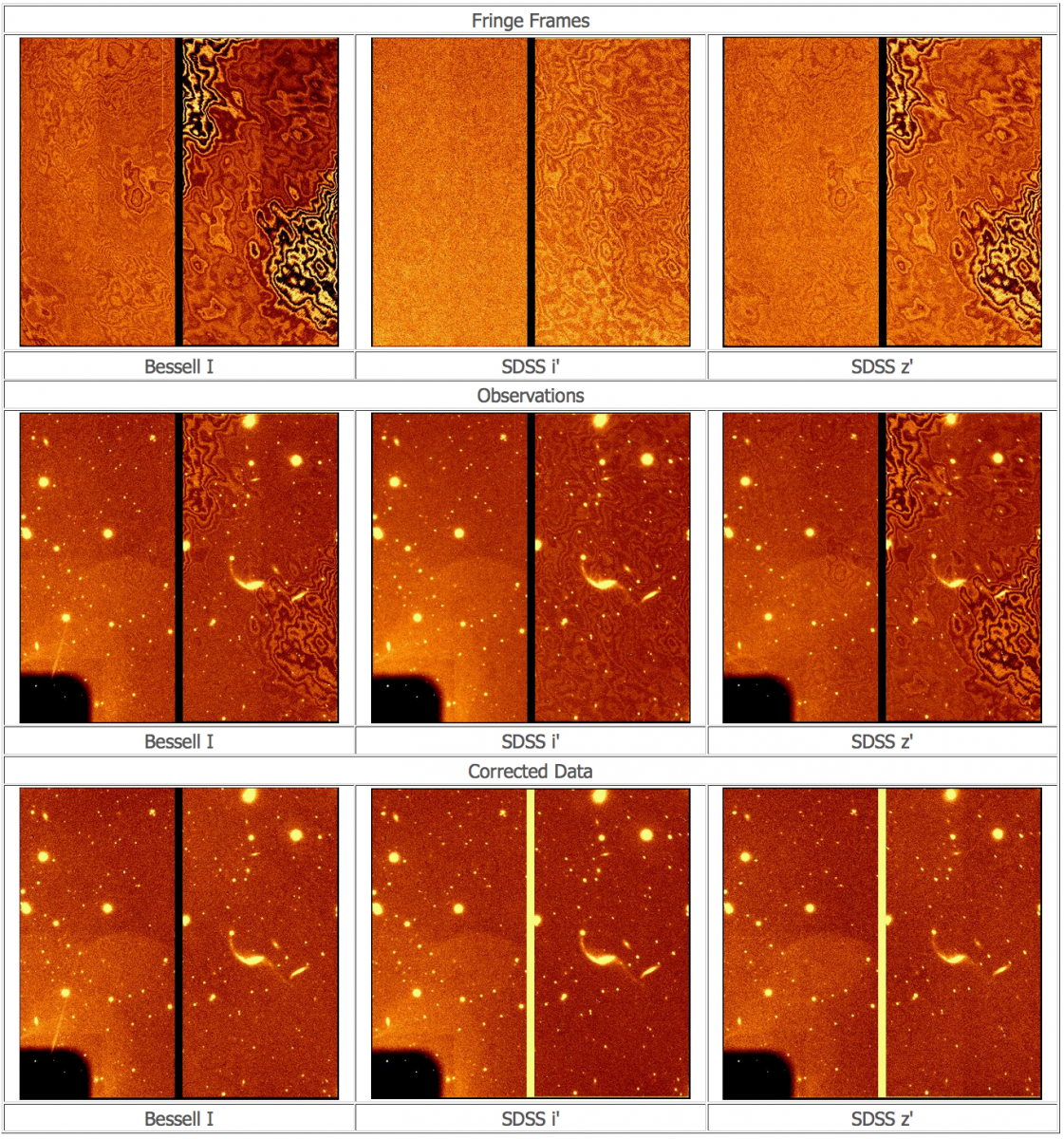
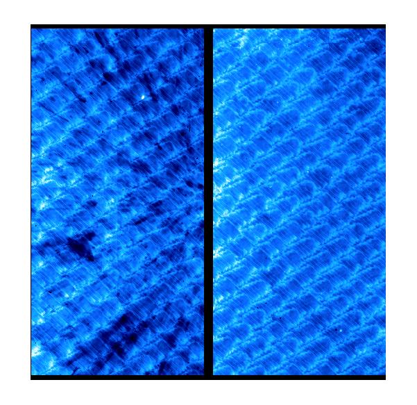
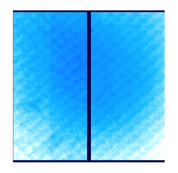
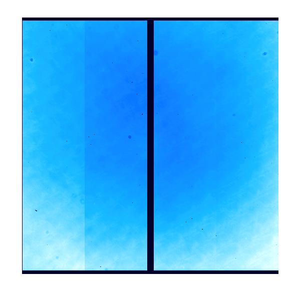
The CCDs show fringing in the I, i' and z' bands (see example here) [33] at the 10%, 3% and 12% level, respectively. In the U band some hatched structure is seen but this flat fields out perfectly. Here are examples of flatfields at the Bessell U [34], B [35], V [36], R [37], and I [38] bands (click the band to see the link).
Ghosts, stray light etc..:
The use of interference filters - which select their passband by reflecting the rest of the light - results in haloes around bright sources. These haloes look like images of the entrance pupil of the telescope with the secondary mirror spider clearly visible, especially when the seeing is good. We have some stray light from encoders in the SOI rotator on the CCDs in the I band. The level is about 0.2 ADU per second, or less than 1% of the dark sky background. We are working on eliminating this stray light. A complete report on these and other optical effects in the SOI is given in a report, available here.
Read-out:
The chips are read out by two amplifiers each. Various read-out and binning modes will be available. Note that a seeing disk of 0.45" is still well-sampled by 2x2 binned pixels, so that only for the very best seeing and using the tip-tilt mode should the CCDs be used in unbinned mode. At present, the tip-tilt mode is not yet offered. SOI is no longer offerred in slow read-out mode (as of 2008 Nov).
Focusing:
Focusing of the SOI is done by charge shifting on the CCD, and moving the telescope focus between steps by automatic software. The number of steps, step size, and exposure time per subexposure can be chosen by the observer.
Guider:
The instrument incorporates a fast readout CCD guide camera which can be used to drive the telescope's tertiary mirror in order to partially compensate atmospheric Tip and Tilt, and correct telescope tracking jitter. The actual performance of this system has yet to be determined, but it is expected that Tip-Tilt correction will be possible with guide stars as faint as R=14, with useful guiding performance down to R=19. The field of view of the guide camera is only 7" square, however, the probe can be placed anywhere within a 12 arcmin diameter patrol field. Normally the probe should be kept outside the central 6x6 arcmin to avoid blocking part of the science field. However, when the best possible Tip-Tilt correction is required it may be desireable to select a guide star close to the science target accepting the obstruction of parts of the field.
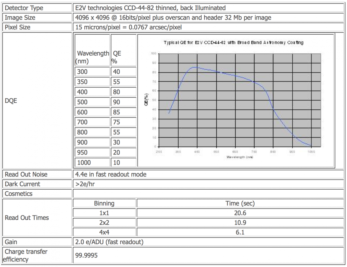
The SOAR Optical Imager is a mini-mosaic comprised of two 2048x4096 E2V CCDs (4096x4096 pixels total). At the bent-Cassegrain port, the pixels subtend 0.0767 arcsec on the sky, providing a field of view 5.25 arcmin on a side.
The CCDs are read by two Leach controllers through 4 amplifiers (2 amps per CCD). Depending on binning and the gain setting, the CCDs can be read in as little as 6.1 seconds (4x4 fast readout) to as long as 106.0 seconds (1x1 slow readout). Please see the table given in the SOI Overview page for a more detailed description. The data are taken and examined via vncviewers on the SOI data acquisition computer (currently known as soaric1). From soaric1, one can transfer the data to their home institution.
Unbinned SOI images plus overscan and header information are approximately 37 Mbytes each. Most normal observations are performed in 2x2 binning mode with a binned pixel size of ~0.15 arcsec and are approximately 9 Mbytes each. A typical night produces about 2 Gbytes of data and easily transferred over the internet. This is the preferred method of the SOAR partners. If this is unfeasible, please contact Sean Points prior to your run so that other options can be discussed.
The SOI filter cartridges contain space for 4 filters, plus one blank position, so that up to 8 filters can be installed in the instrument at the same time. Filters may be up to 100mm square and up to 10mm thick. Smaller filters may be accommodated with special adapters but must be at least 64mm square to avoid vignetting.
Philosophy and Structure of this Manual
This manual is intended for an observer planning to use the SOAR Optical Imager (SOI). It is not intended to serve as a hardware or software reference document describing the inner working of SOI, although some details at that level may appear to help the observer plan observing strategies. Also, we assume that the observer is already familiar with CCD cameras, observations, and data reductions.
The SOI Overview [1] is at the front of this manual. If you've read this far, and don't plan to read any further, be sure you understand the SOI Overview [1] pages.
This manual follows the outlines of the KPNO and CTIO Mosaic imager manuals. Therefore, we have also adopted the philosophy of bald-faced plagarism and have kept structure of those documents. We have made changes to reflect the differences of the SOI mini-mosaic to the KPNO and CTIO Mosaic imagers. We will update this version as improved data and information become available.
Development of the SOAR Optical Imager system is a continuing process. Throughout the lifetime of the instrument, filters will be added, old ones replaced, and software enhanced. This manual represents the status as of the date on the cover page. We expect to revise the manual occasionally to include information gained during engineering runs, as well as to reflect new filters.
Other useful information regarding the use of Mosaic, CCDs, and observing and reduction software can be found at:
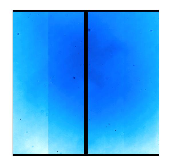
The SOAR Optical Imager (SOI) features two 2048 (serial or pixels/row) x 4096 (parallel or pixels/column) 15 micron per pixel CCDs arranged as a 4096 x 4096 pixel detector. The CCDs are read out through two amplifiers per chip simultaneously using an SDSU-2 Leach controller. The gap between the CCDs is kept to about 102 pixels in the row direction (see Figure 2 showing an image labeled with chip numbers). We have populated the SOI with thinned, back illuminated E2V CCDs. These chips have only minor flaws which have little effect on their scientific performance.
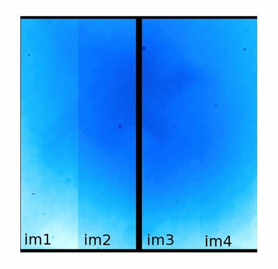
Figure 2: A flat-field (R band) map of the SOI CCDs with their FITS extensions (im1, im2, im3, and im4) labeled accordingly.
Figure 3 shows the average QE of the SOI CCDs.
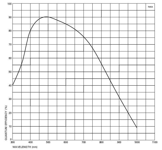
Figure 3: The average E2V CCD QEs.
The SOI dewar contains a highly polished aluminum vessel (11.6 liters) that can be filled with LN2 to 50% capacity via an axial tube and a hold time of 30+ hours. The LN2 can is connected to the CCD mount by a copper braid which has had its thermal resistance optimized. The CCD mount is a kinematic design, with a frame coupled to the dewar front face by G-10 stand-offs. The frame in turn carries the CCD mount and the heater, which is servoed to keep the CCD at a constant temperature to within 0.2 degrees C. The SOI dewar is the smaller blue cylinder on the right-hand side of Figure 4. It is filled by an observing technician at the start of each night.
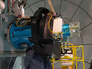
Figure 4: The SOI system mounted on one of the bent-Casseagrain foci of the SOAR Telescope. The dewar containing the 2 CCDs is the smaller blue cylinder located on the right. The SDSU Leach controller is the silver boxr located in front of the dewar.
The two CCDs are read out by an SDSU-3 Leach controller (see Figure 4), connected to a PC running GNU/Linux through a PCI board in a PCI-GNU/Linux-LabVIEW environment. The read-out time using two amplifiers per CCD is 20 seconds in unbinned mode with a 4.4e read noise. Other modes of operation are given in the SOI Overview document at the beginning of this manual. Data values are stored as 16-bit unsigned integers.
The shutter is a single blade "focal plane" type driven by a dc servomotor via a cogged belt. It is low profile (4.7mm) and high performance. Minimum exposure time is less than 200 msec and repeatability below 0.5 msec. The drive profile is trapezoidal. The shutter has been subject to extensive lifetime tests without degradation.
Filters are mounted in two filter cartrides each with space for 4 filters, plus one blank position, so that up to 8 filters can be installed in the instrument at any time. Although the cartridges were designed to be easily removeable, the process of changing them out still requires at least 30 minutes, and we currently have no spare cartridges. Thus it is strongly recommended that users design their programs to avoid filter changes during the night. Filters may be up to 100mm square and up to 10mm thick. Smaller filters may be accommodated with special adapters but must be at least 64mm square to avoid vignetting. To see the list of the currently available filters, together with transmission curves, click HERE [31]. Filters from the CTIO filter list [41] are also available.
The tip-tilt guider consists of a probe containing a miniature (10 mm side) right angled prism which diverts a small portion of the input beam to a second prism, where the beam relay optics send it to the tip-tilt guider detector. The prism size and probe arm cross-section are small (the latter has a cross-section of only 5 mm) because the prism and probe arm may need to occult the science beam if the guide star is desired, or can only be found, close to the field center. The probe assembly is mounted on a Parker-Daedalus XY-stage, with 0.5 micron resolution. It is also possible to fine-tune the focus independently from the telescope focus. The detector system is a thinned, quad-readout Marconi CCD-39 that is thermoelectrically cooled and operated by an SDSU Leach controller in frame-tansfer mode.
The rotator mechanism is driven by a servo motor, directly coupled to a Harmonic Drive gear reduction. This turns a bronze friction wheel against a larger steel wheel which houses a 4-point ball bearing that is attached to the rotating part of the instrument. Position sensing is achieved by a tape encoder located inside the bearing housing. It has a resolution of 0.16 arcsec, more than needed. The rotator has a maximum rotation speed of 0.48 degrees per second and has redundant limit switches for safety. The cable-wrap consists of a IGUS energy chain system, specially manufactured for this application. It is lubricated with Teflon to reduce friction.
All elements of the focal reducer are held in individual cells. The triplet is held by 8 preloaded spring elements with hard points only in the axial direction. The compression of the spring elements was calculated to achieve an acceptable centering. The other two cells are of the "finger" type commonly used in CTIO instruments.
The Atmospheric Dispersion Corrector
The atmospheric dispersion corrector (ADC) incorporated into the SOI is a two-prism linear "trombone-like" design, such as that adopted for the FORS instrument on the VLT. This design is particularly well suited for and alt-azimuth telescope as the angle between the image plane (i.e., the telescope altitude plane) and the atmospheric dispersion axis remains constant for all zenith distances, thus avoiding the need for prism rotation. This holds for any instrument, as is the SOI, mounted on the telescope tube. Our ADC consists of a pair of fused silica prisms with the same apec angle and a constant 180 degree orientation offset. The forward prism corrects for atmospheric dispersion by moving longitudinally in the beam and the fixed prism corrects for the image plane tilt. An image shift occurs depending on the prism separation that can be compensated for by the telescope pointing model.
At present the ADC is not used during SOI observations.
/soar/sites/default/files/SOI/soiobs1.jpg [42]Logging on to the Data Acquisition and Data Analysis Computer
The data acquisition and preliminary reduction computer is called soaric1. A number of different ways to logon to this machine exist, depending upon your preference. These methods are discussed below.
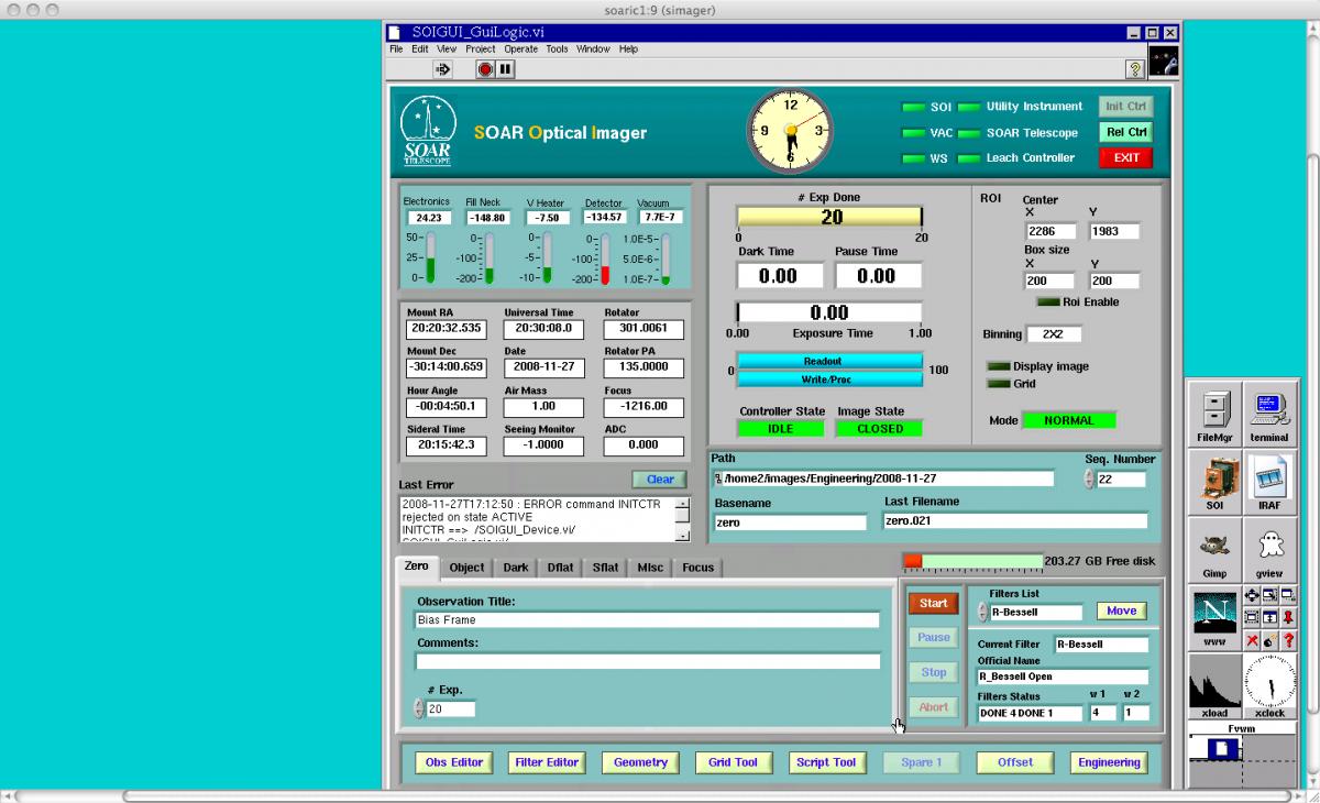
In most cases the GUIs should be started and you will be presented with a data acquisition screen and data analysis screen as shown in Figure 5.
 [42] [42] |
 [43] [43] |
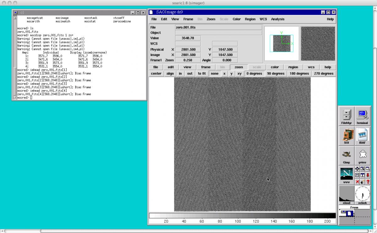
Figure 5: The SOI Data Acquisition and Data Analysis GUI windows.
Starting and Stopping the Data Acquisition GUI
If the data acquisition GUI has not been started, then one should see a light blue screen in the soaric1:9 VNC window with an xload and xclock window that has 8 buttons labeled FileMgr, terminal, SOI, IRAF, Gimp, gview, www, and some window manager utilities. To start the data acquisition software:
If the data acquisition GUI needs to be stopped:
Starting and Stopping the Data Analysis GUI
The SOI data analysis VNC window (soaric1:8) has the same base layout as the SOI data acquisition VNC window (soaric1:9). If the data analysis windows are not up, you will see the xload window and the accompanying buttons described in the data acquisition GUI startup section. Single click on the IRAF button and an IRAF window will open. You will want to open a DS9 window from within IRAF and load the mscred IRAF package.
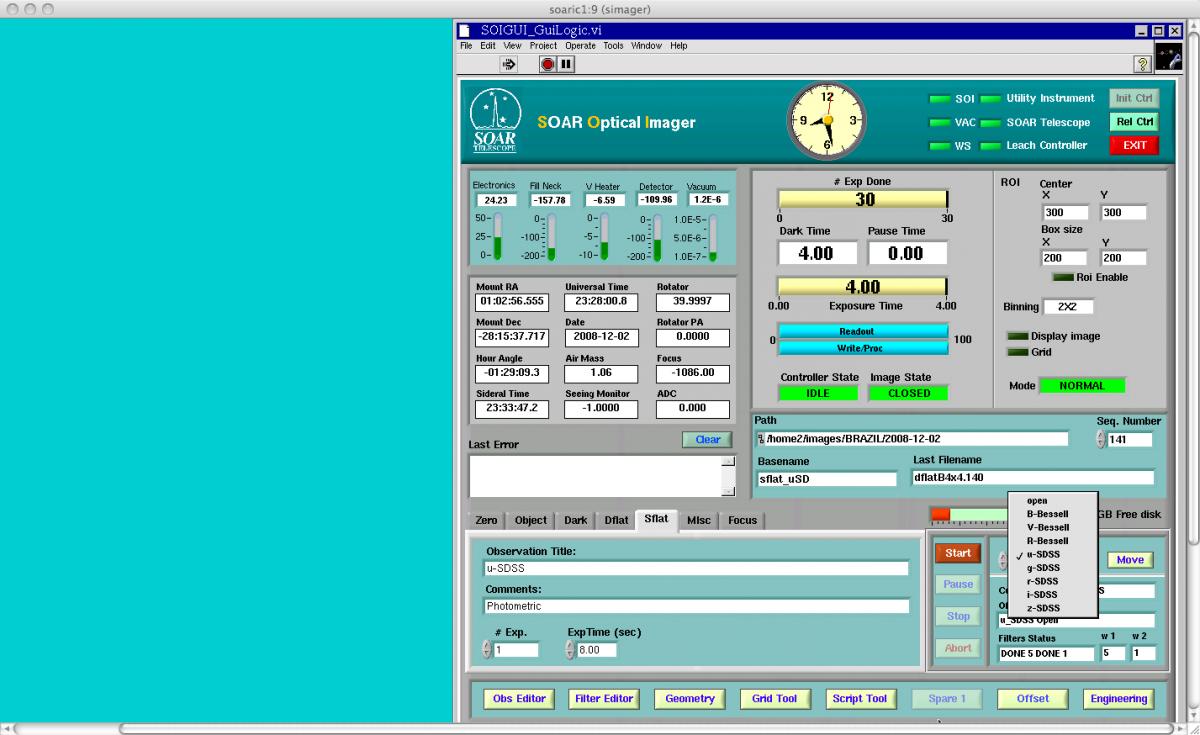
All observing with the SOAR Optical Imager (SOI) is handled through the Data Acquisition GUI. Upon successful startup of the SOI data acquisition GUI on soaric1:9, one should see that the SOI data acquisition window looks something like that shown in Figure 5.
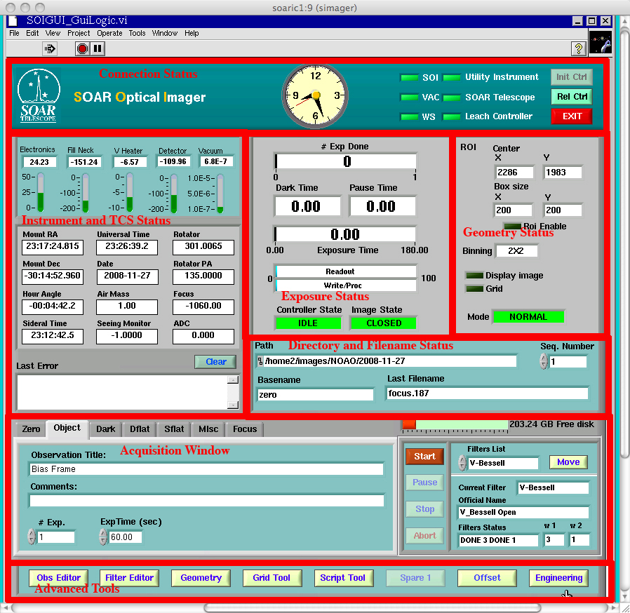
The SOI observing GUI can be divided into certain distinct regions as shown in Figure 6. These include the:
 [44]
[44]
Figure 6: The SOI data acquisition GUI with regions demarcated and labeled.
These OBSTYPEs can be chosen by clicking on the appropriate tab in the upper left-hand side of this section of the GUI. In general, these tabs allow an observer to input the image title and an additional comment to the FITS header. All of the tabs that permit an observer to change the OBSTYPE of an image allow the observer to also change the exposure time of the image, except for a ZERO or Bias Frame observation. Furthermore, if the OBSTYPE is selected to be a DFLAT (Dome Flat), the observer is allowed to turn on and set the intensity of the White Spot Lamps. The Telescope Operators can provide you with the correct intensity values and exposure times for your Dome Flat observations. The "Misc" and "Focus" tabs in the Data Acquisition Region are not currently supported.
Also included in the Data Acquisition section of the SOI GUI are the Start, Pause, Stop, and Abort buttons. Pressing the "Start" button will begin the process of taking an exposure of the currently selected OBSTYPE. During an exposure, one may also click on the "Pause", "Stop", or "Abort" buttons. The "Pause" button will suspend an ongoing exposure until the "Resume" button is clicked. During this time, the shutter should close so that the detectors are no longer integrating on the sky, but the detectors will continue to accumulate cosmic ray hits and dark current. Upon clicking the "Resume" button, the shutter will open and the exposure will proceed as scheduled. Clicking the "Stop" button during an exposure will close the shutter, readout the CCDs, and write the data to the disk. Clicking the "Abort" button will close the shutter and discard the current image. The "Abort" button does not write data to the disk.
Finally, on the right-hand side of the Data Acquisition Region, the observer can select the filter to used during the current observation. To change a filter:
 [45]
[45]
Figure 7: The SOI filter select interface.
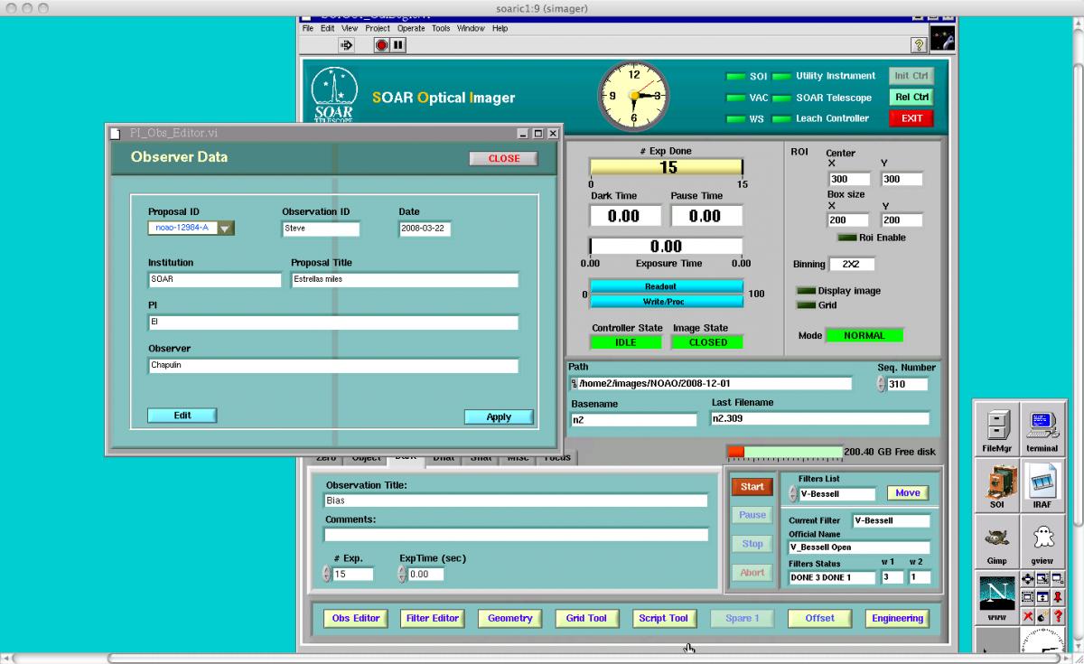 [46]
[46]
Figure 8: The SOI Observer Information interface.
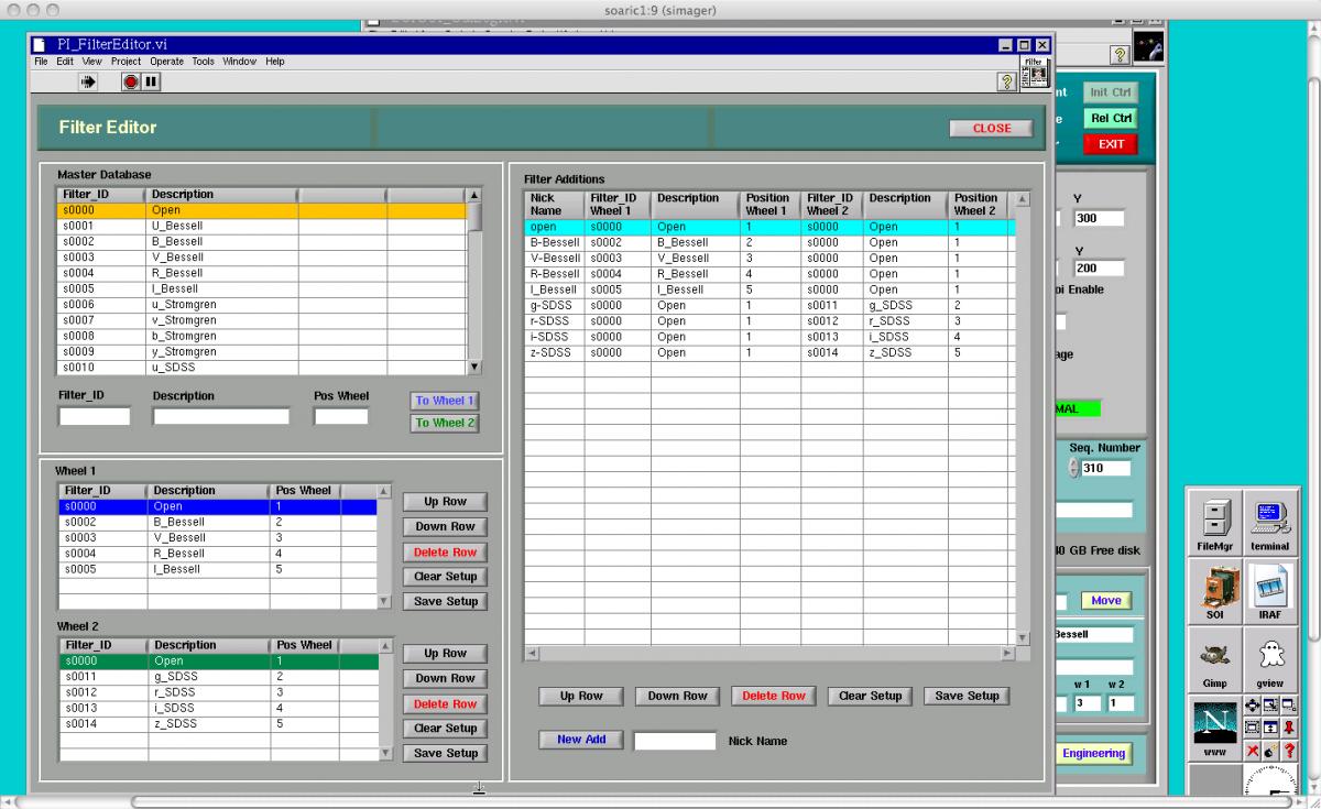 [47]
[47]
Figure 9: The SOI Filter Editor interface.
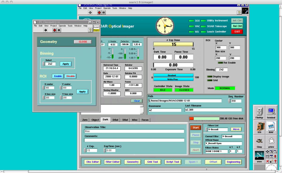 [48]
[48]
Figure 10: The SOI Geometry Editor interface.
To change the binning, click on the Binning "Select" Box. The available options will be shown to you. To finalize your binning selection, click the "Apply" button to the right of the selection box. You should notice that Binning indicator in the Geometry Status section of the GUI flashes from yellow to red during this change. The background of the Binning indicator will remain white after the binning has successfully changed.
To change the Region-of-Interest (ROI) readout of the CCDs, one must first enable the ROI dialog by clicking on the "ROI Enable" button on the Geometry Editor screen. After pressing the ROI button, you can enter the detector coordinates (x,y) and the size in (x,y) of the ROI. The detector coordinates are related to the current binning. Thus, for a 2x2 binned observation, the center of the detector is at (x,y) = (1024,1024).
 [49] [49] |
 [50] [50] |
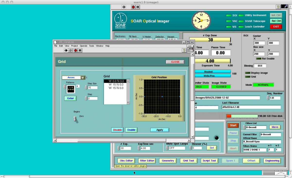
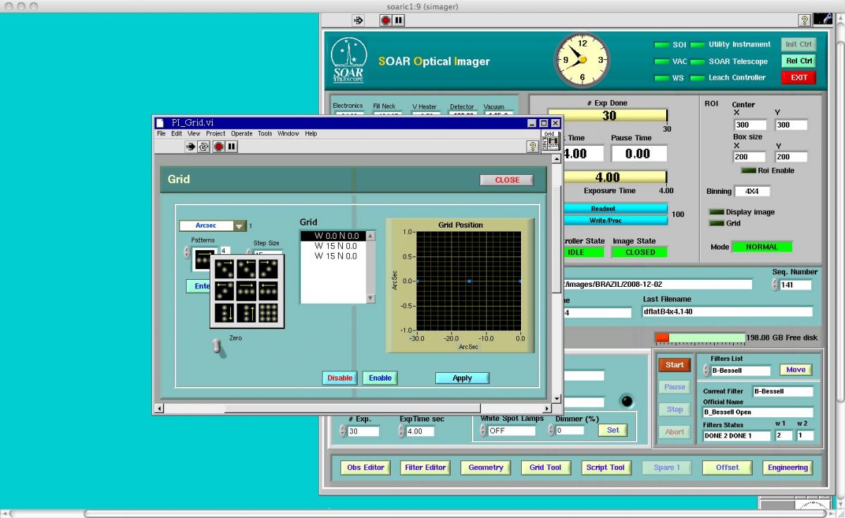
Figure 11 : The SOI Grid Tool Interface.
In order to apply a a dither pattern to the Grid Tool, one should
Prior to your run at SOAR with the Optical Imager, you should have completed the Instrument Setup Form [51]. When using SOI, it is important to send in this form well ahead of time so the proper filters [31] can be installed before your run. In the instrument setup form you can also specify what binning you will use during your run. The default readout is for 2x2 binning with fast readout. Information on the gain settings and readout noise for various binning options under fast readout can be found in the SOI Overview.
In addition to filling out the Instrument Setup Form [51], visiting observers should read the SOAR Visiting Astronomer´s webpage [52] for general information about traveling to and within Chile. Furthermore, visiting investigators should fill out the Travel Information Questionaire [53] so that your transportation and lodgings can be arranged.
Observing logs for your run can be downloaded here [54].
Setting Up for the Start of Your Night/Run
Before you begin observing with SOI, you should first make sure that the data acquisition GUI and the data analysis GUI are running as shown above in Figure 5. If these GUIs are not running, please refer to the sections of this manual about Starting and Stopping the Data Acquisition GUI [18] and Starting and Stopping the Data Analysis GUI [19]. If you have problems with starting either of these, please contact the Telescope Operators or the SOI instrument scientist (Sean Points). They will be able to help you with this task.
After the GUIs are running, you should check that:
You are now ready to use the SOAR Optical Imager. Information on how to takes exposures can be found in Basic GUI Layout [20] section.
You can also look at the step-by-step SOI Observer's Cookbook [30]for help on observing with SOI
At the end of your observing night, please fill out the End-of-Night [55] report for the telescope. Please make note of any problems that were encountered during the night so that they may be resolved before the next night's observing.
Also, at the end of your night observing with SOI, you may want to transfer your data back to your home institution. To do so, open a Terminal window in either the Data Acquisition GUI or the Data Analysis GUI. Once the Terminal window is open, change directories to where your data are located on soaric1. You may then use scp at the shell prompt to copy the data to your home institution.
After your run is complete, please fill out the End-of-Run [56] report.
In this section we discuss the software and observing procedures needed for the following:
Observers familiar with CCD cameras, images obtained using the NOIRLab Mosaic cameras, and the IRAF reduction and analysis software for the most part will find the processing of SOI images to be familiar. At the same time, there are some differences that we touch upon briefly here. To start with, SOI images are recorded in a special multi-extension FITS format (MEF). In brief, the SOI CCDs are saved as individual images grouped together as separate entities in a larger FITS file; only at the end of the reduction are the CCDs assembled as a single large astronomical image. Because of this special format, most IRAF routines will not work directly on the full SOI files. To provide for processing of the SOI format, as well as reduction and analysis tasks specific to SOI, we use some of the MSCRED IRAF routines that were developed for the Mosaic cameras in addtion to having developed some SOI specific IRAF routines. Almost all of the software tasks that we discuss below presume that you will be working within this environment.
A key factor that drives both the data taking and reduction of SOI images is the presumption that the final astronomical exposure will be built from a number of SOI images obtained by dithering the telescope. This places strong demands on the quality of the data reduction to ensure the uniformity of the photometric response of the reduced image. We have custom scripts we use for reducing SOI data; please contact the SOI instrument scientist [57] (Sean Points) to obtain, install and run them on your system.
NOTE: These packages have been quasi-independently developed by astronomers at SOAR, CTIO and MSU. They contain slightly different versions of the same tasks. So it is recommended to download one or the other packages, but not both. For non-expert IRAF MSCRED users, it is advised that the MSU routines be downloaded.
Working with SOI/MEF Data Files
An excellent summary of the MSCRED reduction routines is provided in the two guides written by Frank Valdes: Mosaic Data Reduction System [58] and the Guide to the NOAO Mosaic Data Handling System [59]. The latter link is available in the IRAF/MCSRED package by the command "help mscguide". We encourage SOI users to read through these documents before attempting to reduce their data for the first time. These guides also provide a thorough description of all MSCRED tasks that may be of use during the night's observing.
The SOAR Optical Imager data format is a multi-extension FITS (MEF) file. The file contains five FITS header and data units (HDU). The first HDU, called the primary or global header unit, contains only header information which is common to all the CCD images. The remaining four HDUs, called extensions, contain the header and images from the four amplifiers on the two CCDs.
The fact that the image data is stored as FITS format images is not particularly significant. A single FITS format image file may be treated in the same way as any other IRAF image format. The significant feature is the multi-extension nature of the data format. This means that commands that operate on images need to have the image or images within the file specified. Only commands specifically intended to operate on MEF files, such as those in the MSCRED package, can be used by simply specifying the file name. Commands that operate on files rather than images, such as copying a file, may be used on MEF files. In general, it is safest to use only MSCRED commands on MEF files. IRAF V2.11 is required to run MSCRED. The basic syntax for specifying an image in a MEF file to an IRAF task is:
filename.fits[extension]
where "filename" is the name of the file. The ".fits" extension does not need to be used. The "extension" is the name of the image. For the SOI data the 4 CCD images have the names "im1" through "im4" (but the simple "1" through "4" works, too). The extension position in the file (where the first extension is 1) may also be used. To access the global header (for listing or editing) the extension number is 0; i.e. filename.fits[0].
There is currently no wildcard notation for specifying a set of extensions. So to apply an arbitrary IRAF command that takes a list of images you must either prepare an @list (or type the list explicitly) or use the special MSCCMD command. The task MSCCMD takes an IRAF command with the image list parameter replaced by the special string "$input". The input list of SOI files will then be expanded to a list of image extensions.
Displaying and Evaluating SOI Images at the Telescope
During observing, a small set of IRAF commands are commonly used to examine the data. This section describes these common commands. While this section is oriented to examining the data at the telescope during the course of observing, the tools described here are also used when reducing and analyzing the data at a later time.
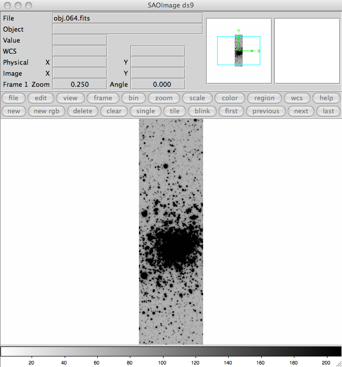
The two IRAF commands DISPLAY and MSCDISPLAY are used to display the images in DS9. DS9 and an IRAF command window should be running on the data analysis GUI [19]. The DISPLAY task is used to display individual images - in this context, the individual amplifiers in a SOI exposure designated by the appropriate extension ID. There are many display options that are discussed in the help page that will not be discussed here. The only special factor in using this task with the SOI data is that you must specify which image to display using the image extension syntax discussed previously. As an example (see Figure 12), the central portion of extension im2 (i.e., AMP#2) in displayed in the first frame of a DS9 window using the IRAF DISPLAY command and the whole image is displayed in the second frame of a DS9 window using the IRAF MSCDISPLAY command:
 |
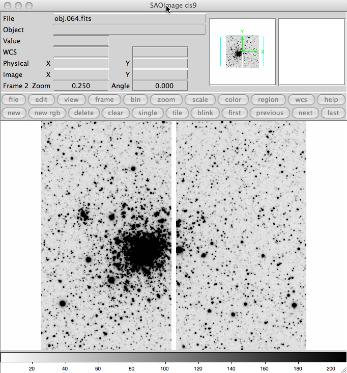 |
Figure 12: (left) A DS9 image display of the second SOI amplfier using the IRAF DISPLAY command. (right) A DS9 image display of an entire image using the IRAF MSCDISPLAY command.
The MSCDISPLAY task is based on DISPLAY with a number of specialized enhancements for displaying MEF data. It displays the entire MEF observation in a single frame by "filling" each image in a tiled region of the frame buffer. The default filling (defined by the order parameter) subsamples the image by uniform integer steps to fit the tile and then replicates pixels to scale to the full tile size. The resolution is set by the frame buffer size defined by the "stdimage" variable.
Many of the parameters in MSCDISPLAY are the same as DISPLAY and there are also a few that are specific to the task of displaying a mosaic of CCD images. The mapping of the pixel values to gray levels includes the same automatic or range scaling algorithms as in DISPLAY. This is done for each image in the mosaic separately. The new parameter "zcombine" then selects whether to display each image with it's own display range ("none") or to combine the display ranges into a single display range based on the minimum and maximum values ("minmax"), the average of the minimum and maximum values ("average"), or the median of the minimum and maximum values. The independent scaling may be most appropriate for raw data while the "minmax" scaling is recommend for processed data. Another new optional answer here is "auto", which is the default, will try to use the best option, given the status of the data.
During your nightly observing, MSCDISPLAY is normally used during image acquisition to insure that your object is centered at the desired location and that it does not lie in the chip gap between the CCDs. In order to measure the delivered image quality of an exposure, one normally uses the IRAF DISPLAY and IMEXAM commands to measure the FWHM and the ellipticity of stars in the field. The FWHM can be compared to the seeing reported by the Cerro Pachón seeing monitor (you need to be connected to the VPN to access this link) [60]. If the measured image quality is consirably worse than the site seeing, you may want to re-tune the mirror. Another measure of the image quality is the ellipticity of stars in the observed field. If the ellipticity, as measured by the IMEXAM command, is greater than 0.15 you may want to re-tune the mirror. The telescope operators normally tune the mirror at the beginning of the night. After that, it is the observer's responsibility to check the image quality and request that the mirror be re-tuned.
Calibration Data to Obtain at the Telescope
In general the only calibration data that one needs to obtain at the telescope are Bias frames, and Flats (Dome and/or Twilight Sky). These data are obtained by clicking on the appropriate tab in the Data Acquisition Region of the Data Acquisition GUI [20]. This will set the proper "OBSTYPE" keyword (i.e., ZERO, DOMEFLAT, or SKYFLAT) in the FITS headers for your calibration data.
Click here for table of exposure times and lamp intensities [61] that will allow you to take dome flats with a peak intensity of ~20000 counts for most filters. When taking twilight sky flats, one should start observing as soon as you can after sunset, and take at least 5 twilight sky flats per filter. As soon as the peak counts for a particular filter are below ~30000, we recommend taking a series of exposures until either the peak counts drop below ~10000 or you have enough twilight sky flats to reduce your data.
Fringing with SOI
The only other calibration data one will likely need to obtain at the telescope are sky frames for fringing correction. As any thinned, back illuminated chip the SOI E2V devices suffer from considerable fringing in the Bessel I, SDSS-i and SDSS-z bands [62]. Fringing is most evident in longer exposures. Depending on the nature of your science targets you can take either of two approaches to approach obtaining the fringing correction images:
1) If your field is sparse and contains mostly/only stars (maybe a few faint, small galaxies), then you can use the same science frames to construct the master fringe removal frame. All that is needed is to carry out the observation as a series of dithered/offset observations, which you will later median-combine without registering (after the basic bias subtraction and flatfielding). This will eliminate all stars and leave only the sky background with the fringe pattern - see the examples in this page. [63] Just make sure you dither/offset by at least 10 arcsec between each exposure.
2) If you are imaging an extended object which covers a significant part of your field, like a large galaxy, or you are looking at a very crowded stellar field, the previous approach will not work. In this case you should offset to a nearby "empty" field (sparse stellar field) to take your sky data. Again, you need to split your total exposure time among at least 3, preferably 5 exposures, that you will then median-combine; dither at least 10 arcsec between each frame. Ideally, your total "empty" sky image should have an integration time equal to your science frame.
It is important to bear in mind the the fringing pattern will not be the same across all the sky or all position angles, so for the best fringe removal, you should create the master fringe frame using either the same science data or images obtained in the same general area of the sky.
Removal of the fringing pattern is done by applying the master fringe frame as an illumination correction to the data that have been already bias-subtracted and flatfielded.
More details can be found in these links on fringing correction:
This section assumes that either the NOIRLab SOI reduction package or the MSU SOI reduction package has been downloaded and successfully installed on your local reduction computer. If not, please contact the SOI instrument scientist [57] (Sean Points) for help.
The first step in reducing SOI data should be to perform the BIAS scan and TRIM section corrections. The values for BIASSEC and TRIMSEC are given in the FITS headers for each amplifier. Please see the IRAF MSCRED CCDPROC help pages for further information. After all of the images are Bias-subtracted and Trimmed, the Zero (or Bias) frames should be combined into a master bias for the night using the IRAF mscred.zerocombine task. After this step, the flats and object images should be Zero-corrected by setting the appropriate flags in mscred.ccdproc. Combine the dome flats and if necessary twilight flats, depending on the filter. Apply the Flat-field correction for your data using mscred.ccdproc. You should now be ready to perform photometry on your SOI data.
Step-by-step instructions on reducing SOI data can be found here [68].
Here we provide our users with Typical Exposured Times used in Dome Flats for SOI and SAMI. The values are not precise but are meant to give the astronomer an idea.
Please click here for a printable PDF file with the filters and exposure times. [61]
Links
[1] http://www.ctio.noirlab.edu/soar/content/soi-overview
[2] http://www.ctio.noirlab.edu/soar/content/introduction-soi
[3] http://www.ctio.noirlab.edu/soar/content/introduction-soi#Overview
[4] http://www.ctio.noirlab.edu/soar/content/introduction-soi#Philosophy
[5] http://www.ctio.noirlab.edu/soar/content/introduction-soi#Supplemental
[6] http://www.ctio.noirlab.edu/soar/content/soi-hardware
[7] http://www.ctio.noirlab.edu/soar/content/soi-hardware#H1
[8] http://www.ctio.noirlab.edu/soar/content/soi-hardware#H2
[9] http://www.ctio.noirlab.edu/soar/content/soi-hardware#H3
[10] http://www.ctio.noirlab.edu/soar/content/soi-hardware#H4
[11] http://www.ctio.noirlab.edu/soar/content/soi-hardware#H5
[12] http://www.ctio.noirlab.edu/soar/content/soi-hardware#H6
[13] http://www.ctio.noirlab.edu/soar/content/soi-hardware#H7
[14] http://www.ctio.noirlab.edu/soar/content/soi-hardware#H8
[15] http://www.ctio.noirlab.edu/soar/content/soi-hardware#H9
[16] http://www.ctio.noirlab.edu/soar/content/soi-software
[17] http://www.ctio.noirlab.edu/soar/content/soi-software#S1
[18] http://www.ctio.noirlab.edu/soar/content/soi-software#S2
[19] http://www.ctio.noirlab.edu/soar/content/soi-software#S3
[20] http://www.ctio.noirlab.edu/soar/content/soi-software#S4
[21] http://www.ctio.noirlab.edu/soar/content/soi-software#S5
[22] http://www.ctio.noirlab.edu/soar/content/soi-software#S5a
[23] http://www.ctio.noirlab.edu/soar/content/soi-software#S5b
[24] http://www.ctio.noirlab.edu/soar/content/soi-software#S5c
[25] http://www.ctio.noirlab.edu/soar/content/evaluating-and-reducing-soi-images
[26] http://www.ctio.noirlab.edu/soar/content/evaluating-and-reducing-soi-images#R1
[27] http://www.ctio.noirlab.edu/soar/content/evaluating-and-reducing-soi-images#R2
[28] http://www.ctio.noirlab.edu/soar/content/evaluating-and-reducing-soi-images#R3
[29] http://www.ctio.noirlab.edu/soar/content/evaluating-and-reducing-soi-images#R4
[30] http://www.ctio.noirlab.edu/soar/sites/default/files/SOI/soi_tutorial_Oct2015.pdf
[31] http://www.ctio.noirlab.edu/soar/content/filters-available-soar
[32] http://www.ctio.noao.edu/noao/content/CTIO-3x3-inch-and-4x4-inch-Filters
[33] http://www.ctio.noirlab.edu/soar/sites/default/files/images/Instruments/soi_fringe_frames.png
[34] http://www.ctio.noirlab.edu/soar/sites/default/files/images/Instruments/FlatU.jpg
[35] http://www.ctio.noirlab.edu/soar/sites/default/files/images/Instruments/FlatB.jpg
[36] http://www.ctio.noirlab.edu/soar/sites/default/files/images/Instruments/FlatV.jpg
[37] http://www.ctio.noirlab.edu/soar/sites/default/files/images/Instruments/FlatR.jpg
[38] http://www.ctio.noirlab.edu/soar/sites/default/files/images/Instruments/FlatI.jpg
[39] http://www.noao.edu/kpno/manuals/dim/
[40] http://www.noao.edu/kpno/mosaic/mosaic.html
[41] http://www.ctio.noao.edu/noao/content/Filters
[42] http://www.ctio.noirlab.edu/soar/sites/default/files/SOI/soiobs1.jpg
[43] http://www.ctio.noirlab.edu/soar/sites/default/files/SOI/soiiraf1.jpg
[44] http://www.ctio.noirlab.edu/soar/sites/default/files/SOI/soiobs3.jpg
[45] http://www.ctio.noirlab.edu/soar/sites/default/files/SOI/filtermove1.jpg
[46] http://www.ctio.noirlab.edu/soar/sites/default/files/SOI/obsdata1.jpg
[47] http://www.ctio.noirlab.edu/soar/sites/default/files/SOI/filtereditor1.jpg
[48] http://www.ctio.noirlab.edu/soar/sites/default/files/SOI/geometry1.jpg
[49] http://www.ctio.noirlab.edu/soar/sites/default/files/SOI/grid3.jpg
[50] http://www.ctio.noirlab.edu/soar/sites/default/files/SOI/grid5.jpg
[51] http://www.ctio.noao.edu/SOAR/Forms/INST/setup.php
[52] http://www.ctio.noirlab.edu/soar/content/visiting-astronomers-guide
[53] http://www.ctio.noao.edu/travel/itinerary.php
[54] http://www.ctio.noirlab.edu/soar/content/soar-observing-logs
[55] http://www.ctio.noao.edu/SOAR/Forms/EON/Form.php?telescope=SOAR
[56] http://www.ctio.noao.edu/new/Tools/Forms/EOR/Form.php?telescope=SOAR
[57] http://www.ctio.noirlab.edu/soar/content/soar-staff
[58] http://iraf.noao.edu/projects/ccdmosaic/Reductions
[59] http://www.ctio.noirlab.edu/soar/sites/default/files/documents/valdes2.pdf
[60] http://139.229.15.76/web/PachonSM/environ_dimm3.php
[61] http://www.ctio.noirlab.edu/soar/sites/default/files/SOI/SOI_Flatfield_Exptimes.pdf
[62] http://www.ctio.noirlab.edu/soar/sites/default/files/SOI/soi_fringe_frames.png
[63] http://www.ctio.noirlab.edu/soar/content/fringing-soi
[64] http://www.ctio.noirlab.edu/soar/sites/default/files/SOI/Basis_for_a_SOAR_optical_imager_pipeline.pdf
[65] https://www.eso.org/sci/facilities/lasilla/instruments/efosc/inst/fringing.html
[66] http://www.noao.edu/noao/noaodeep/ReductionOpt/Skyflat.html
[67] http://stsdas.stsci.edu/cgi-bin/gethelp.cgi?rmfringe
[68] http://www.ctio.noirlab.edu/soar/content/soi-image-reduction