Normal Startup

Check all desktops on the observers console to be sure there is NOT a "TightVNC: ispi's X desktop (ctioa9:9)" already running.

• If there IS NOT already a "TightVNC: ispi's X desktop (ctioa9:9)" running then
  • Single click on the 'ISPI VNC' button on the left of the screen. (IF button doesn't work, then in a terminal window, at the prompt type: display_ispi). This will pop up a vnc view desktop.  The desktop will have an xload window with 4 buttons. One of these is labeled 'ArcVIEW.'
  • Single click on the 'ArcVIEW' button. This will pop up the ISPI Control GUI (with the really cool cross section view of ISPI), and an 'ArcVIEW Main Application' window.  The Application window should have two round buttons, labelled 'Connected?' that appear red.
  • On the  ISPI Control GUI, there is a white arrow icon in the upper left corner of the window. Single click on the white arrow. This arrow should now turn black. The two buttons in the Application window should turn green.
  • Minimize the Application window by clicking on the underscore '_' icon on the blue bar, in the upper right corner of each window.  You are now ready to operate ISPI.

• If there IS already a "TightVNC: ispi's X desktop (ctio:9)" running, it can be in a couple of states:
  • There is only the gray desktop with an xload window that has  4 buttons labelled ArcVIEW, IRAF, Vacuum and terminal If this is the case:
    • Single click on the 'ArcVIEW' button. This will pop up the ISPI Control GUI (with the really cool cross section view of ISPI), and an 'ArcVIEW Main Application' window.  The Application window should have two round buttons, labelled 'Connected?' that appear red.
    • On the  ISPI Control GUI, there is a white arrow icon in the upper left corner of the window. Single click on the white arrow. This arrow should now turn black. The two buttons in the Application window should turn green.
    • Minimize the Application window by clicking on the underscore '_' icon on the blue bar, in the upper right corner of each window. You are now ready to operate ISPI.

• The ISPI Control GUI (with the really cool cross section view of ISPI) is already displayed on the desktop. In this case, Check the color of the arrow icon in the upper left corner of the ISPI Control GUI window.
  • If the arrow is white then Single click on the white arrow. This arrow should now turn black. The two buttons in the Application window should turn green.
  • If the arrow is black then you are already ready to operate ISPI, however CHECK the 'ArcVIEW Main Application' window to see that the 'Connected?' buttons are green. If you cannot see the 'ArcVIEW Main Application' window, you can find or open it by clicking on the bar at the bottom of the VNC desktop window.

July 07, 2005; Bob Blum

Quick Reference [1]

Observing Sequences

• ISPI data taking may be "scripted" and complete sequences executed through the ISPI GUI.

• Several examples are available (H [2], J [3], K [4]). Each line of the text file corresponds to a single image written to disk. The key elements are filter changes (one filter per sequence in these examples), exposure time and coadds where exposure*coadds is the total time per image, and the resulting image is the sum of the number of coadds specified. For example, a 10 sec exposure of 3 coadds would produce one image with a total of 30 seconds. The image would be the sum of three 10 second frames. Currently Fowler samples, a type of read mode to reduce noise, are always set to 1. The offsets specify the dither pattern to use and can be either absolute or relative, the choice being made by selecting a button on the GUI itself.

  See /home2/ispi/observers/ on the ISPI computer for many more example sequences. Any of these can be loaded directly into the instrument control GUI by clicking on the load button in the Sequence Control panel of the GUI. Use the dialog to navigate to the ascii text file of choice.

• Modify existing sequences by first making a copy. Each observer may create a sub-directory in /home2/ispi/observers/ to save their sequences. These will not be deleted.

• Each step of the sequence needs to have the same number of fields (see the GUI) even if nothing is changed during that step (e.g. the filter). It is best to copy existing sequences and modify them as needed rather than starting from scratch.

• Use care with the focus sequences as the f/8 focus mechanism has been known to go to the wrong position.

Focus

• Obtaining a good focus takes practice. The main cause of focus changes is due to systematic temperature changes of the telescope truss. The change in focus due to temperature is -1000 steps/C for the f/8 focus used by ISPI (go to higher focus numbers as the temperature gets colder).

• One can monitor the temperature by typing "temp4m" on a terminal on the observers console (not on the vnc session connected to ctioa9). Use one of the "upper truss" readouts.

• The focus can be changed by using the TCS focus control on the ISPI System Control GUI (lower left of main GUI). Click on the button to set the value entered in the box. Do not send a "0" value to the focus. Look on the TCS status monitor (an independent CRT usually to your left). Find the current focus (something like 185,500 at 10C), and enter that value to start.

• To find the best focus when you have no idea what it is, first use the last value from the previous night and estimate the change due to the difference in last night's temperature and the current temperature. Ask the night assisitant if you don't know these values. Next, begin a run of up to 10 images, each with a focus change of 1000 steps. The estimate for the best focus should be image five or six. The first image should be the farthest "in" and you should take successive images going "out" to higher numbers, each time entering a new focus in the System Control portion of the GUI. Analyze all the images, and set the final focus by first going "below" the target value and then moving the final small amount (say 200 steps) to the target by going out against gravity.

• Once a rough focus is set by the above procedure, a better focus can be found by repeating the procedure with a step of 200 units and 5-6 images.

• At the beginning of the night, the temperature can change significantly during the time it takes to set the focus. Beware.

• Always set the desired focus by moving out against gravity to avoid backlash.

• On the IRAF display, an out of focus image is typically elongated. For images which extend from upper left to lower right, focus should be adjusted to higher numbers. Go to lower numbers for images extended upper right to lower left. Use caution here since telescope motion or other problems could be confused with focus. At some point near focus, the image shape is not a good indicator of which way to adjust.

Detector Characteristics, Linearity, and Saturation

• Detailed linearity behavior is shown here [5].

• Keep ISPI counts below about 10000 ADU for data which are ~/< 1% non-linear, or 20000 ADU for data ~/< 2%.

• Hard saturation will occur at about 40000 ADU.

• The ISPI gain is 4.25e-/ADU.

• The ISPI dark is ~0.1e-/sec for long exposures.

• When changing filter or exposure time, the first one or few images will exhibit differing bias structure. This is a feature of the array. It means the first images will have poor background subtraction relative to others in the sequence. If this is important, plan to take one or more "junk" frames.

Flat Fields

• Check here [6] for information on how to take flats.

• The dome flat field lights are activated from control boxes in the computer room. Have the support astronomer or telops staff show you where the controls are and how to operate them. You will typically use only a single set of lamps controlled by the "bottom" box (of three).

• Typical exposures will be 3-10 sec with the lamp control set to 3 amps.

Disk Space

• Please write images to /home2/ispi/images/. You may make a subdirectory here of your choosing, e.g. 20040728/.

• It may be necessary to backup some of your data and then delete it to make room for the rest of your run.

• Your data are archived every night incase of a backup or disk failure. This archive is not user accessible. Contact telops or the support scientist if you have had a data disaster.

• You should have the entire set of data for your run backed up when you leave the mountain. After that, it may be deleted any time.

Observing Efficiency

• For K-band images, the background will set the maximum observing time. Depending on the ambient temperature this could range from about 15 to 30 seconds.

• Use coadds to increase efficiency. Coadding images uses less time than writing the same number of separate images and dithering the telescope. I.e. for a given total exposure time, integrate as long as possible on each frame, take the minimum number of dither positions, and coadd as necessary.

• Experience shows ISPI is about 60% efficient for 60 second K-band images (20 seconds by 3 coadds) and 10 dithers typically less than about 60''.

February 3, 2005

The following summarizes some issues regarding flat fields taken with ISPI using the Ks (aka KA) and H (aka (HA) filters (J band results are expected to be similar to those for H).

• These data were taken on 7 May 2004.
  • The dome flats use the lower lamp box at 3.00 amps
  • Exposure times are 3.3s, 5s, and 10s, for Ks, H, and J, respectively (15 frames lights on, 15 frames lights off)
  • Sky flats below were made from 100 data frames at 3.3 seconds (with rejection of 30 high and 20 low frames from the stack to account for stars in the field).
• Ideally, flats should be constructed from series of "illumination on" minus "illumination off" images.
• In all cases, flats should be made from series of frames with the exact same data taking parameters (exposure time, coadd, repeats, Fowler reads, etc).
• Dome flats are recommended for Ks band data.
• Sky flats made from data (i.e. observations) will probably work equally well as dome flats for J and H.
•     Twighlight flats will probably give similar results for H and J as for dome flats. At Ks, twighlight flats with varying illumination in which the "low" frames are subtracted from the "high" frames might give similar (or even better) results as for Ks dome flats.
•     Twighlight flats at Ks made by subtracting dark frames will probably give similar results as for the sky flats described below and these will not be as good as dome flats.

The following plots show the results of placing a star at 100 evenly spaced positions over the ISPI 2048x2048 detector under photometric conditions.

• The individual frames were flat fielded with either a dome flat (as made in bullet 2 above) or a sky flat made by combining the data and subtracting a dark frame from the result.
• All flats were fixed for bad pixels and normalized by the mean counts in the image.
• Photometry is for a 6 pixel aperture with a 3 pixel sky annulus with inner radius of 6 pixels. No particular effort was made to optimize the aperture for varying image quality.
• Normal dome flats at Ks or dome/sky flats at H (and probably J) should have large scale uncertainties of about ~/< +/- 3% over the full field of view.
• The Ks flats might be affected by extra emission arising from the warm structure around M3 and a possible undersize of M3. The difference between "on" and "off" images appears to account for this putative extra emission. Sky flats would not normally account for such emission, and this is a possible explanation for the apparent better accuracy seen below for dome vs sky flats.
• It is not known what produces the residual large scale flat fielding errors seen in the plots.
• The following table contains text files of the photometry results which can be used to estimate second order corrections to H and Ks flats.

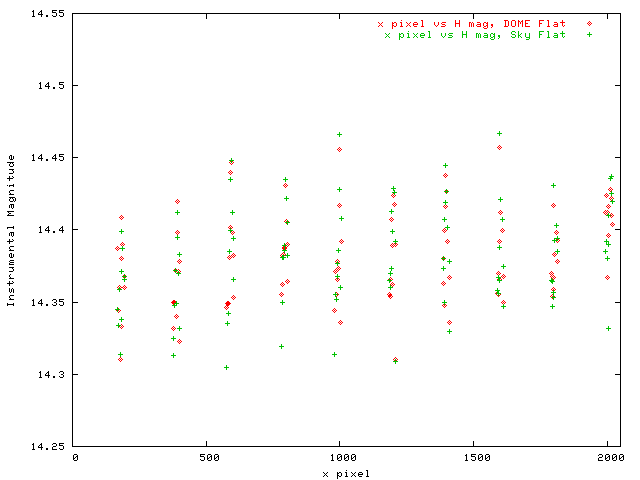
Figure 1a. Instrumental H Magnitude vs x pixel. Both sky and dome flats give similar results.

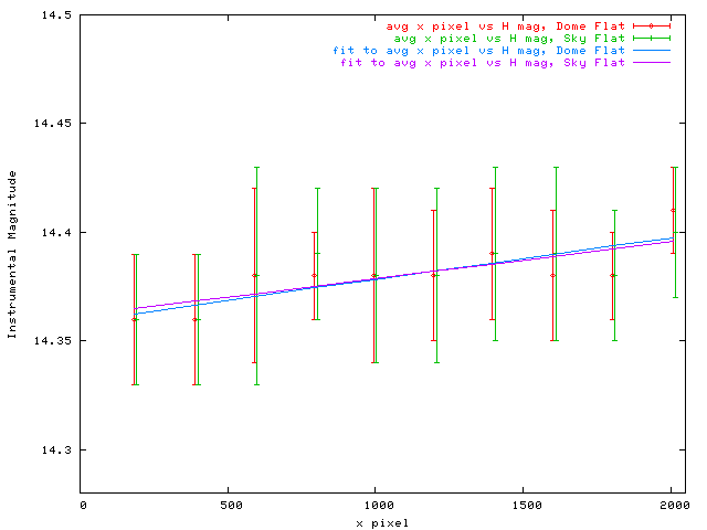
Figure 1b. Instrumental H Magnitude averaged over all y pixels for given x pixel. The linear fit suggests a full range of variation of +/- 2% due to large scale flat fielding uncertainty.

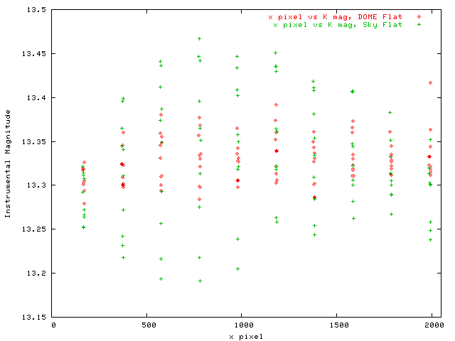
Figure 2a. Instrumental Ks Magnitude vs y pixel. The sky flat shows a much larger range of values than the dome flat. These represent systematic changes in the flat field, not variations due to photon statistics. Sky flats made by using illuminated frames and a dark frame should not be used unless the region of interest for objects and standards is restricted. The differences here are probably due to vingetting of the field at M3 combined with "off M3" background at Ks.

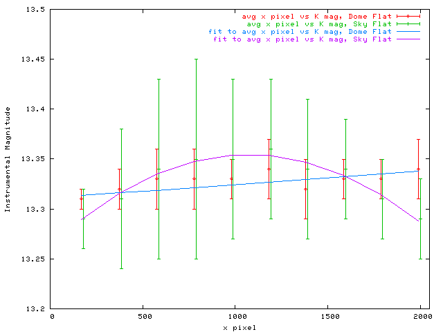
Figure 2b. Instrumental Ks magnitude averaged over all y pixels for a given x pixel. The fits show that the sky flat probably contains a component of emission comming in at the edges of the field around M3. The beam from M3 is "suppressed at the edges" by the flat.

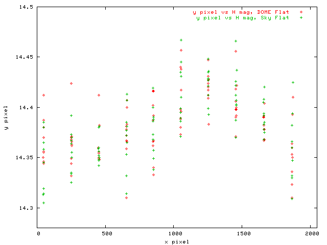
Figure 3a. Same as Figure 1a, but for the y pixel vs H.

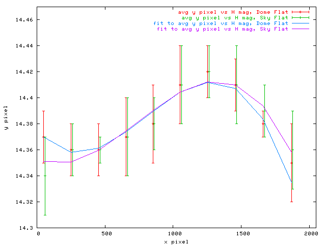
Figure 3b. Same as Figure 1b, but for y pixel vs H. The large scale variations are well fit by a 3rd order polynomial.

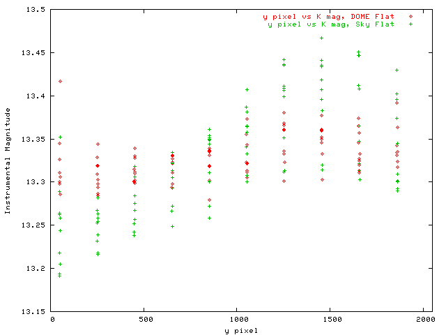
Figure 4a. Same as Figure 2a, but for the y pixel vs Ks.

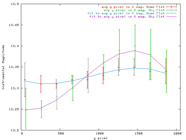
Figure 4b. Same as Figure 2b, but for y pixel vs Ks.
 

A nonlinearity correction has been derived for ISPI data. This is an average correction based on all pixels. A series of J-band frames interleaved with minimum exposure dark ("bias") frames were used to derive the correction. The dark following each illuminated frame was subtracted from that illuminated frame.

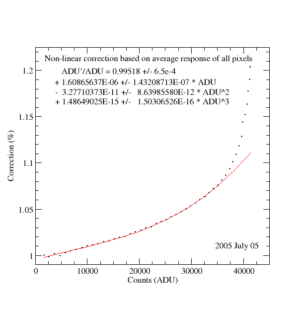
The correction was derived by considering a linear fit to the counts vs exposure time for counts < about 7000 ADU. The residual of this linear fit, normalized by the fit value, plus one was then fit to a third order polynomial. The IRAF coefficients (see IRAF irlincor) are available through the cirred [19] data reduction package in the task "osiris.cl".

Last Update 06 July, 2005; Bob Blum

Basics

ISPI data should be flat fielded and sky (and/or "dark") subtracted. These steps can be accomplished with may standard IRAF or IDL routines. One way is to use the basic reduction tool "osiris" provided in the cirred [20] set of IRAF scripts. A basic set of initial reduction steps would include:

• Build flats from raw ISPI images, typically subtracting a combined "lights off" image from a combined "lights on" image. Use the cirred task med.cl (for "median combining").
• Build a bad pixel mask from images with typical bad pixels (for example, use a lights on image and a lights off or dark image). Use the cirred task maskbad.cl.
• Run the cirred meta script "osiris" to read in a series of images efficiently, divide each by a flat, and fix bad pixels (interpolates over bad pixels in x and y). For ISPI, choose flipy=yes. This puts N up and E to the left on an IRAF image display and is required to run the astrometric tools described below. If a bad pixel mask called "mask.fits" was created, and a flat called "flat.fits", then a typical osiris call might be:

  cl> osiris n1 n2 pre=r suf=n mask=mask.fits div=yes, dome=flat.fits

  n1 and n2 are command line params, the others can be set in the param file. Here pre is a "prefix" or image base name, suf will be the output image suffix and the images to be reduced have numbers n1 thru n2, inclusive. Suppose the prefix for input images is "r" for raw. If n1=1, and n2=3, then images r001.fits, r002.fits, r003.fits will be processed and images r001n.fits, r002n.fits, and r003n.fits will be output. Look over the cirred pages, the osiris param file, and the osiris.cl script itself for more information.

• The flat fielded images should be sky subtracted. Separate dark subtraction is not needed as long as the images are not scaled during sky subtraction. If images are to be scaled significantly, and the dark and bias pattern is important compared to the sky level, then darks of the same exposure and coadds should be subtracted before sky subtraction (usually at the very beginning; this can be done in osiris.cl). Use the cirred script sky_sub. A typical sky_sub might be:

  cl> sky_sub 10 25 sky=kskyimage make+ sub+

  Where the image numbers work as in the osiris example. Prefixes and suffixes are set in the param file or on the command line. The two flags "make" and "sub" control how sky_sub behaves. Make will combine the indicated images into a sky frame, and sub will subtract that sky frame from the images. A set of independent skys could be combined with make+ ans sub- (to suppress subtraction) and applied to a separate set of object frames with make- (to suppress making of the sky frame) and sub+.

Astrometry

One of the most important tasks for ISPI data reduction is the assignment of a proper coordinate system and correction of image distortions. These tasks are conceptually straightforward, but often difficult to accomplish in practice (especially the latter). A preliminary set of tasks and scripts has been set up to allow for the determination of the world coordinate system keywords to be included in the image headers. A solution to higher order distortions is also available, which will allow for the registration and combination of dithered images.

Software.

The processing of ISPI images described here requires that one download and install several external packages.

• WCSTOOLS [21]. These are C libraries and programs by Douglas Mink at the SAO. These routines update the headers of ISPI images with FITS keywords describing the image coordinate system, its projection on the sky, etc. Install the WCSTOOLS software, and read the information about imwcs [22] which is the program used to compute a coordinate solution and update the image headers.

• Catalogs. WCSTOOLS needs an astrometric reference catalog. These can be existing catalogs like 2MASS or user catalogs. The best way to proceed is to download and install one or more catalogs locally. At CTIO, we have so far experimented with 2MASS, since this is very useful for near infrared observations in the Galactic plane. Other catalogs will work well for regions where the optical extinction is not high. To install the 2MASS catalog, follow the instructions given by the WCSTOOLS pages [23]. The disk space requirement is about 40 GB.

• A program to find image centroids in the ISPI images. This can be accomplished in IRAF (for example daofind). Other well known programs are DOPHOT, DAOPHOT, and SExtractor [24]. Finding accurate centroids is necessary for certain options using WCSTOOLS.

• A program to resample or interpolate images. We have used SWARP [25], a program by Emmanuel  Bertin.

Updating the Basic Headers for a WCS.

• The images should be preprocessed to have a near zero rotation from some known position. For ISPI, the usual N up E left projection is easily accomplished by choosing the "flipy" flag in the osiris.cl IRAF meta script. ISPI raw images have N down and East left when displayed in IRAF. An EPOCH keyword should also be added to the header which matches the value of the ISPI EQUINOX keyword (the default is 2000.0).

• The simplest task needed for raw ISPI images is to add appropriate world coordinate system (WCS) keywords [26]. The program imwcs should be used to do this. There are a variety of options, but a simple call would be the following:

  > imwcs -c tmc -d t150s.dao -h 200 -n 6 -vw -p 0.303 t150s.fits

  In this example, -c tmc calls for the 2MASS catalog. The location of the catalog is specified during the build process of WCSTOOLS. -h 200 calls for 200 stars to be used in the matching between the image and catalog, and -n 6 refers to the order of the fit between image and catalog positions (6 parameters in each axis). -p 0.303 gives the initial image scale in arcseconds per pixel for ISPI; this is required since this information is not in the header. Alternately, one could add SECPIX (with a value of 0.3) to the ISPI image headers. -d t150s.dao specifies that the file "t150s.dao" be used for the input x,y positions of the stars to be matched by the catalog. This file should be sorted on brightness so the brightest stars are used. The file should be one star per line, x, y, and mag. "#'s" indicate comments and are ignored in this file, as are any fields after the first three of each line. See the IMWCS Command Line Arguments [27] for more information. -vw sets the "verbose" flag along with a call (w flag) to write a new image (in this case t150sw.fits) which has the updated WCS. See the imwcs command line argument -o for more output options, including updating the input image header.

• The result of IMWCS is an image updated (if desired) with a WCS which is a standard tangent plane projection on the sky. In the above example, a new image t150sw.fits was created from t150s.fits. The pixel data are not changed, only the header.

• Once this step has been performed, use DS9 (SAO image) to display the updated image. The WCS coordinates should appear in the upper left of the image display. WCS specific IRAF scripts or any other program which is based on the FITS standard should also now be able to read and use the WCS information stored in the updated ISPI header.

Taking Distortion into Account

• The above call to imwcs results in a new image header, but it is often desired to actually resample or interpolate the image to a new projection. This could just be to have the pixel to sky projection modified or to allow for correcting higher order distortions. The latter is the case for ISPI since these distortions will affect the combination of dithered images. ISPI exhibits distortion, so combining dithered images without correcting for this will result in a degraded PSF at positions away from the center of the image. The effect can be significant (of order several pixels change in FWHM.
• The key to creating a plate solution which accounts for the ISPI distortions is to have an image or images with many stars across the field of view and a set of accurate catalog positions.
• Once a matched catalog of pixel and sky coordinates is in hand, any program which fits the latter to the former and writes an appropriate solution can be used to further update the image header. In practice, our solution relies on the IRAF task "ccmap" because this task will do the fit and add the appropriate keywords to the header. This is done in the IRAF TNX [28] system. The advantage is that the SWARP [25] program used to resample the dithered ISPI images automatically handles the TNX system (which is not officially part of the FITS standard). TNX is a combination of the linear WCS solution plus higher order terms. The fit is a general polynomial in x and y with cross terms. Initial testing with ISPI suggests ccmap fits of 4th-6th order (in IRAF speak) with full cross terms do well.

In this image, the residuals to a linear fit are shown. The peak errors in position would be about three pixels if the distortion were not accounted for. In the next image, the residuals for a 4th order fit are shown. The RMS is less than 0.1'' which is about 1/3 of an ISPI pixel.

• The ccmap solution is written to a database file which IRAF understands and also to the image header if the flag "update" is turned on (i.e. set to yes) and images are specified in the images parameter of the task. The image header keywords are explained in the TNX description [28].

• The ccmap solution can easily be applied in SWARP. Refer to the SWARP pages for details on how to execute this program. A simple call to swarp would be:

  > swarp -c swarp.gc t150sw.fits t151sw.fits t152sw.fits t153sw.fits t154sw.fits

  In this example, the swarp config file is "swarp.gc" and five images are reinterpolated. Each image can have its own TNX solution, which in our example would be the combination of WCS and TNX keyword values produced by imwcs and ccmap. Unless the fit to each image is very good, it is advisable to use an average solution for the higher order terms (and rotation and scale in this case). This can easily be done in swarp by specifying an auxillary header file with the FITS keywords and values. Cutting and pasting from the above solution from the FITS header, a file of the form t15?sw.head was made for each image. The file has the following form and is identical for each image:

  WAT0_001= 'system=image'
  WAT1_001= 'wtype=tnx axtype=ra lngcor = "3. 4. 4. 1. -0.09223848232288634 0.095'
  WAT2_001= 'wtype=tnx axtype=dec latcor = "3. 4. 4. 1. -0.09223848232288634 0.09'
  CD1_1   =  -8.4729762794223E-5
  CD1_2   =  7.23448951262463E-7
  CD2_1   =  7.40672424953437E-7
  CD2_2   =  8.47678406227307E-5
  WAT1_002= '30461739012073 -0.08294874238596413 0.086260218248302 -3.81821493608'
  WAT1_003= '0989E-6 0.004201053595244364 0.004530606959289172 -0.722711400721411'
  WAT1_004= '9 -5.887103279160741E-4 0.006853642315098468 0.0766861807819218 0. -'
  WAT1_005= '0.005316483436707363 -0.4617939442868234 0. 0. 0.1156522538399243 0.'
  WAT2_002= '530461739012073 -0.08294874238596413 0.086260218248302 4.34379162931'
  WAT2_003= '0940E-6 -5.007423412969465E-4 6.003889063455503E-5 0.084985861670387'
  WAT2_004= '73 0.003355387441743075 0.003754664665905738 -0.3911461579926636 0. '
  WAT2_005= '0.001750656256554302 0.04350355226749533 0. 0. -0.5986827241716564 0'
  WAT1_006= ' 0. 0. "'
  WAT2_006= '. 0. 0. "'
  END

  These lines were copied directly from the fits header of the image used in our example to find the higher order solution. A tab follows the keyword "END."

• Swarp will combine the dithered images using the individually resampled images (see the swarp documentation and the config file options). The resampling includes rotation, scale, distortion and the standard pixel to sky projection (in this case, the TAN or tangent plane projection).

  Bad pixels may be rejected in the combine process by using the "pixel weighting" capability in SWARP. A simple weighting which rejects bad pixels can be accomplished by using the "mask2.fits" file produced by maskbad.cl (see the cirred package). This file has a 1 for each good pixel and 0 for each bad one. The file is called in the swarp configuration file by specifying its name in the WEIGHT_IMAGE keyword and using WEIGHT_MAP as the weighting method (it appears that one must specify this file name for each input image. I.e, make a coma separated list for the value of WEIGHT_IMAGE with the same file name repeated to match the number of input images). See the swarp documentation for more information. A slightly more sophisticated weight map can be made by multiplying the normalized flatfield image by mask2. Finally, one can specify a unique weight mask for each image through the file "imagename.suffix.fits" where "suffix" is given in the swarp config file, and the default is "imagename.weight.fits."

End to End Processing of ISPI Images

The following is an example of how ISPI images may be fully processed using the tools discussed on this page (cirred, WCSTOOLS, SWARP, IRAF).

1. Make flats: Use med.cl to combine lights on and off images into a domeon and domeff image, respectively. Subtract the off image from the on.
2. Make bad pixel masks: Use maskbad.cl to create bad pixel masks.
3. Fix flats: Use fixfits.f to fix the flat images. The resulting images will have bad pixels interpolated over. If the images are named "dFilterNamef.fits", then the osiris.cl script will apply the right flat according to the FITS header filter name where FilterName is th evalue of this header parameter (e.g. KA for the ISPI Ks filter).
4. Run osiris.cl: The meta script which will preprocess images, divide by a flat, and add appropriate head key words.
5. Sky subtract the images: Use sky_sub.cl to make and subtract sky frames.
6. Add a WCS: Use do_wcs.cl to add a World Coordiante System to the images. (Preliminary script included in cirred package. Requires WCSTOOLS [21]. Requires a catalog implementation for the WCSTOOLS.).
7. Compute high order distortions: Use do_ccmap.cl to compute the high order distortion coefficients and add them to the image header (Preliminary script included in cirred package. Requires WCSTOOLS. Need to incorporate TNX keywords manually as described above).
8. Shift/Combine images: Use SWARP [25] (by Emmanuel Bertin) to reinterpolate the images and optionally shift and combine them.
9. Make a color image: SWARP can be used to shift and orient the final J, H, and K images so they can be combined in a false color image.

Acknoledgements: We would like to acknowledge the useful comments and input of Silas Laycock regarding ISPI data reduction and astrometry. It is also a pleasure to acknowledge the very useful software and documentation of the Mink WCSTOOLS, the Bertin SWARP program, and the IRAF suite.

Please mail questions or comments to:
rblumATctio.noao.edu
nvdbliekATctio.noao.edu
bgregoryATctio.noao.edu

Typically, ISPI observations are short and unguided. This simplifies the execution of large mosaics. If dithering about in a restricted area for a long time, then guiding can be useful to improve or maintain image quality. The guide field is provided by the portion of the telescope field which is viewed "past" the tertiary mirror (M3) which delivers the science field to ISPI by a 45 deg reflection. M3 and the guider both live in the white rotator box fixed to the back of the primary mirror cell.

The M3 mirror as viewed from above. The mirror is actually an elliptical shape but appears round since it is mounted 45 deg to the optical axis. The guide field is to the left in this image.

This sketch shows the available guide field using the F/8 guider. The inner radius is 15.35 arcmin and the outer radius is 23.03 arcmin as measured from the center of the ISPI field. Guide stars should be chosen toward the center of the annulus if possible (i.e. between R3 and R4). This will allow for the guide stage to follow the offsets for dithers of several arcmin. If you need to offset further (e.g. to take separate sky frames), make sure to have the night assistant turn off the guiding before the offset is made. The scale is 6.58 arcsec/mm.

Last Update 21 April, 2005; Bob Blum